Classifying Variables

In our first lesson, we established the two major branches of statistics: descriptive statistics for summarizing your sample and inferential statistics for making conclusions about the wider population. Now, we move from the why of analysis to the what—the data itself. The nature of your data is the single most important factor that dictates the statistical methods you can use.

Today, we will focus on classifying variables, which are the specific characteristics you measure in a study (like age, blood pressure, or treatment group). By the end of this lesson, you will be able to classify any variable you encounter as either categorical (nominal, ordinal) or numerical (discrete, continuous). This skill is not just a theoretical exercise; it is the first and most critical step in choosing the correct statistical test for a research question, a core skill for your work as a biostatistician.

A Framework for Classifying Variables

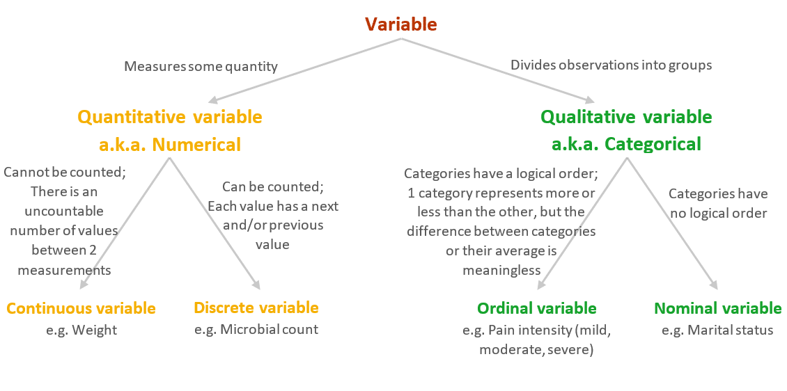
At the highest level, every variable you encounter in medical research can be sorted into one of two families: qualitative (or categorical) and quantitative (or numerical).

Quantitative (Numerical) variables measure a quantity. They answer questions like "how much?" or "how many?" and are expressed as numbers (e.g., patient's weight in kg, number of previous surgeries).
Qualitative (Categorical) variables divide observations into groups or categories. They answer questions like "what type?" and are expressed as labels (e.g., blood type, smoking status).

Within each of these families, there are two important sub-types. The decision tree below provides a clear visual roadmap for classifying any variable. We will refer back to this structure as we explore each type in detail.

This flowchart illustrates the main branching paths for classifying variables. The first split is between quantitative and qualitative data, followed by further classification into continuous/discrete and ordinal/nominal types, respectively.

To ground these concepts in a medical research context, we'll turn to a concise article from the National Institutes of Health (NIH).

The Anatomy of Data - PMC - PubMed Central - NIH

This article provides clear, clinically relevant definitions and examples that are directly applicable to the research papers you will encounter and analyze.

First, read the introductory sections Types of Data to solidify the main distinction between qualitative and quantitative variables. Next, read the section Qualitative Data. Focus on understanding the difference between nominal and ordinal data. Pay close attention to the examples provided, such as sex (nominal) and the ASIA impairment scale (ordinal). Finally, read the section on Quantitative Data. Here, the key is to grasp the distinction between discrete (counts) and continuous (measurements) data.

Reinforcing the Concepts

You've now read the formal definitions. Let's review and reinforce them.

1. Qualitative (Categorical) Variables

These variables place individuals into distinct groups.

Nominal Variables: These are categories without any intrinsic order or ranking. You can't say one category is "higher" or "better" than another.
- Medical Examples: Blood Type (A, B, AB, O), Marital Status (Single, Married, Divorced), Patient Gender (Male, Female), Presence/Absence of a disease (Yes/No).
- When a nominal variable has only two categories (like Yes/No or Male/Female), it is often called a binary or dichotomous variable. This is a very common type in medical research.
Ordinal Variables: These are categories that have a meaningful, logical order, but the intervals between the categories are not necessarily equal or measurable.
- Medical Examples: Pain Scale (Mild, Moderate, Severe), Cancer Staging (Stage I, II, III, IV), Likert scale responses on a questionnaire (e.g., Strongly Disagree, Disagree, Neutral, Agree, Strongly Agree).
- You know that "Severe" pain is worse than "Mild" pain, but you cannot say it is exactly three times worse. The distance between the ranks is not defined.

2. Quantitative (Numerical) Variables

These variables represent measurable quantities.

Discrete Variables: These are numerical variables that can only take specific, distinct values, usually whole numbers. They are often the result of counting.
- Medical Examples: Number of children in a family, number of hospital admissions in a year, number of asthma attacks per week.
- You can have 2 asthma attacks or 3, but you cannot have 2.57 attacks.
Continuous Variables: These are numerical variables that can, in theory, take any value within a given range. They are often the result of a measurement.
- Medical Examples: Height (e.g., 175.5 cm), Weight (e.g., 68.2 kg), Systolic Blood Pressure (e.g., 121.3 mmHg), Serum Cholesterol (e.g., 198.7 mg/dL).
- The precision is only limited by the measuring instrument. Between any two values, an infinite number of other values are possible.

For an engaging review with more practice questions, the following video from Medicosis Perfectionalis, a channel tailored for medical education, is excellent.

Types of Variables - Numerical vs. Categorical - Discrete vs. Continuous - Ordinal vs. Nominal

This video uses a rapid-fire, question-and-answer format that will help you quickly test and solidify your understanding of all four variable types.

Watch the video from the beginning to the end. It starts with the main quantitative/qualitative split and then provides clear definitions and numerous examples for all four subtypes we've discussed. Pay close attention to the practice questions from the series of examples.

From Theory to Practice: Classifying Variables in SPSS

This classification system is the foundation for your work. Your chosen software, SPSS, requires you to correctly define the "level of measurement" for each variable. Getting this right is crucial because SPSS uses this information to determine which analyses and charts are appropriate.

SPSS uses slightly different terminology for its "Measure" column:

Nominal: Same as our definition. Used for unordered categories.
Ordinal: Same as our definition. Used for ordered categories.
Scale: This is SPSS's term for quantitative data. It encompasses both discrete and continuous variables. If a variable is a number you can perform meaningful math on (like calculating an average), you will set it as "Scale" in SPSS.

The following video provides a perfect, concise explanation of how these concepts translate directly into the SPSS software environment.

SPSS: Understand Ordinal, Nominal & Scale (aka Level of measurment)

This video is essential as it bridges the statistical theory with the practical steps you will take in SPSS. It also highlights why incorrect classification can lead to errors.

Watch the video from the beginning, paying special attention to two key parts: The definitions of Ordinal, Nominal, and Scale data as used in SPSS. The explanation of why this matters, from this timestamp. This directly addresses your goal of knowing which tests to use.

To see what this looks like in practice, examine the screenshot of the SPSS "Variable View" below. This is the screen where you define your variables.

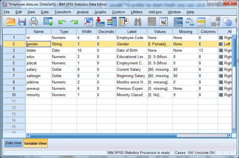
This image shows the "Variable View" in SPSS. Each row represents a variable, and columns define its properties. Note the 'Measure' column on the far right (partially obscured), where you would select Nominal, Ordinal, or Scale.

Let's look at a few variables from the image:

gender: The values are likely coded (e.g., 1=Male, 2=Female). Since there's no order, its 'Measure' would be set to Nominal.
educ: This represents educational level. If coded as 1=High School, 2=Bachelor's, 3=Master's, there is a clear order. Its 'Measure' would be Ordinal.
salary: This is an exact monetary value. It's a quantitative variable. Its 'Measure' would be set to Scale.

Finally, it's worth noting that in data analysis, we sometimes convert quantitative data into categorical data. For example, you might take a continuous variable like 'age' and group it into an ordinal variable: 'Young' (<40), 'Middle-aged' (40-60), and 'Senior' (>60). This is done to simplify analysis or to highlight trends across age groups, but it comes at the cost of losing detailed information.

Conclusion

In this lesson, we have dissected the anatomy of data, a crucial step toward building your biostatistical expertise. Here are the key takeaways:

Variables are broadly classified as Quantitative (Numerical) or Qualitative (Categorical).
Qualitative variables are sub-divided into Nominal (unordered categories, e.g., blood type) and Ordinal (ordered categories, e.g., pain scale).
Quantitative variables are sub-divided into Discrete (countable whole numbers, e.g., number of seizures) and Continuous (measurable values in a range, e.g., blood pressure).
In SPSS, these correspond to three "Measure" types: Nominal, Ordinal, and Scale (which covers both discrete and continuous).
Correctly identifying a variable's type is the non-negotiable first step in selecting the appropriate statistical analysis and graphical display.

You have now learned to distinguish between descriptive and inferential statistics and how to classify the data you'll be working with. In the next lesson, we will add another layer of classification: distinguishing between dependent and independent variables. This final distinction will complete the foundational framework you need to start selecting the right statistical test for a given research scenario.