NFA to DFA Conversion (Subset Construction)

Welcome to your next lesson. In our previous sessions, we explored the world of nondeterminism, defining Nondeterministic Finite Automata (NFAs) and learning powerful strategies to design them. You saw that the "guessing" power of NFAs and the flexibility of ε-transitions often lead to much simpler and more intuitive machine designs compared to their deterministic counterparts.

This naturally leads to a crucial question: are NFAs more powerful than DFAs? Can they recognize languages that DFAs cannot? Today, we will answer this question definitively. The learning outcome for this lesson is to convert an NFA to an equivalent DFA using the subset construction algorithm. By demonstrating that for any NFA, we can construct a DFA that recognizes the same language, we will prove that these two models are equivalent in their computational power. This is a cornerstone result in automata theory.

The Intuition: From Parallel Threads to Deterministic States

Recall the "parallel computation view" of an NFA: when it reads an input symbol, it forks a new thread for each possible transition, maintaining a set of all possible current states. While the NFA itself is nondeterministic because it has choices, the evolution of this set of active states is perfectly deterministic. If you know the current set of active states and the next input symbol, you can predict exactly what the next set of active states will be.

This is the core insight behind the NFA-to-DFA conversion. We will construct a DFA where each state corresponds to a set of states from the NFA. The DFA will deterministically simulate the NFA's parallel execution.

The following video from MIT OpenCourseWare provides an excellent conceptual overview of this idea. The lecturer, Prof. Michael Sipser (author of a classic textbook on this subject), explains why NFAs are not more powerful than DFAs and introduces the idea of the subset construction.

2. Nondeterminism, Closure Properties, Conversion of Regular Expressions to FA

This video explains the equivalence of NFAs and DFAs and introduces the subset construction algorithm conceptually.

Please watch the segment from the introduction of the theorem to the explanation of how DFA states correspond to subsets of NFA states. Focus on the main idea: the DFA keeps track of the set of possible states the NFA could be in.

The Subset Construction Algorithm

Let's formalize the construction. Given an NFA $N = (Q, Σ, δ, q_{0}, F)$ , we will construct an equivalent DFA $D = (Q^{'}, Σ, δ^{'}, q_{0}^{'}, F^{'})$ . The key is defining the components of $D$ in terms of $N$ 's components.

1. The States of the DFA ( $Q^{'}$ )
The states of our new DFA will correspond to subsets of the NFA's states. Theoretically, the set of states $Q^{'}$ is the power set of $Q$ , denoted $P (Q)$ . If $N$ has $n$ states, $D$ could have up to $2^{n}$ states. In practice, we only care about the states reachable from the start state.

2. The Start State of the DFA ( $q_{0}^{'}$ )
The NFA starts in state $q_{0}$ . However, it can immediately take any number of ε-transitions without consuming input. Therefore, the initial state of the DFA must represent all states the NFA can be in before reading the first symbol. This set is called the ε-closure of $q_{0}$ .

ε-closure(S): For a set of NFA states $S$ , ε-closure( $S$ ) is the set of states reachable from any state in $S$ by following zero or more ε-transitions.

So, the start state of our DFA is $q_{0}^{'} = ε-closure ({q_{0}})$ .

3. The Accepting States of the DFA ( $F^{'}$ )
The NFA accepts if any of its parallel threads ends in one of its accepting states $F$ . Therefore, a state in our DFA (which is a set of NFA states) is an accepting state if it contains at least one accepting state from the NFA.
$F^{'} = {R \in Q^{'} ∣ R \cap F \neq = \emptyset}$

4. The Transition Function of the DFA ( $δ^{'}$ )
This is the heart of the algorithm. To compute the transition $δ^{'} (R, a)$ for a DFA state $R \subseteq Q$ and an input symbol $a \in Σ$ , we follow a two-step process:

First, determine all possible states the NFA can move to from the states in $R$ after reading $a$ . Let's call this set $S$ . Formally, $S = ⋃_{q \in R} δ (q, a)$ .
Second, account for any subsequent ε-transitions. The new DFA state is the ε-closure of $S$ .

Therefore, $δ^{'} (R, a) = ε-closure (⋃_{q \in R} δ (q, a))$ .

The following resource provides the formal definitions for the subset construction.

Introduction to Theory of Computation Equivalence of DFA ...

These lecture notes from UC Merced give a concise and formal definition of the resulting DFA.

Please read the section titled "Formal Construction". The notation \hat{\Delta}(q, a) used here represents the set of states reachable from state q on input a, which implicitly includes handling the ε-closure. The definition of Q', q'_0, F', and \delta' provides the rigorous foundation for the algorithm. The correctness proof that follows is also valuable for your mathematical interest, though we will focus on the application.

A Practical Walkthrough: Incremental Construction

Building a DFA with $2^{n}$ states and then pruning unreachable ones is inefficient. Instead, we can build the DFA on-the-fly, discovering new states as we compute transitions. This is often called the incremental subset construction.

Let's apply this to convert the following NFA, which recognizes the language (a|b)*abb, into a DFA.

An NFA with states {0, ..., 10} and ε-transitions that recognizes strings ending in `abb` preceded by any combination of `a`'s and `b`'s.

Let the NFA be $N = (Q, Σ, δ, q_{0}, F)$ where:

$Q = {0, 1, ..., 10}$
$Σ = {a, b}$
$q_{0} = 0$
$F = {10}$
$δ$ is given by the diagram.

We will build the transition table for the equivalent DFA, $D$ .

Step 1: Determine the start state of D
The start state is $ε-closure ({0})$ . Following all ε-paths from state 0, we can reach states 1, 2, 4, and 7.
So, $q_{0}^{'} = ε-closure ({0}) = {0, 1, 2, 4, 7}$ . Let's call this new DFA state A.

Step 2: Compute transitions for state A
We start with our first (and currently only) state, A.

On input 'a':
1. From states in A, where can a lead? Only state 2 has an a-transition, to state 3. So, the intermediate set is ${3}$ .
2. Now compute $ε-closure ({3})$ . From 3, we can reach 6, and from 6 we can reach 7, 1, 2, and 4.
3. So, $δ^{'} (A, a) = ε-closure ({3}) = {1, 2, 3, 4, 6, 7}$ . This is a new state. Let's call it B.
On input 'b':
1. From states in A, where can b lead? Only state 4 has a b-transition, to state 5. The intermediate set is ${5}$ .
2. Now compute $ε-closure ({5})$ . From 5, we can reach 6, and from 6 we can reach 7, 1, 2, and 4.
3. So, $δ^{'} (A, b) = ε-closure ({5}) = {1, 2, 4, 5, 6, 7}$ . This is another new state. Let's call it C.

Our DFA transition table so far:

State	Name	on 'a'	on 'b'	Final?
{0,1,2,4,7}	A	B	C	No

Step 3: Compute transitions for new, unexplored states (B and C)
Now we process state B = {1, 2, 3, 4, 6, 7}.

On input 'a': From B, state 2 goes to 3, and state 7 goes to 8. Intermediate set: ${3, 8}$ . $ε-closure ({3, 8}) = ε-closure ({3}) \cup ε-closure ({8}) = {1, 2, 3, 4, 6, 7} \cup {8} = {1, 2, 3, 4, 6, 7, 8}$ . Let's call this new state D.
On input 'b': From B, state 4 goes to 5. Intermediate set: ${5}$ . $ε-closure ({5}) = {1, 2, 4, 5, 6, 7}$ , which is state C.

Next, we process state C = {1, 2, 4, 5, 6, 7}.

On input 'a': From C, state 2 goes to 3. Intermediate set: ${3}$ . $ε-closure ({3}) = {1, 2, 3, 4, 6, 7}$ , which is state B.
On input 'b': From C, state 4 goes to 5. Intermediate set: ${5}$ . $ε-closure ({5}) = {1, 2, 4, 5, 6, 7}$ , which is state C itself.

We continue this process for each new state we discover (like D), until no new states are generated. The process is deterministic and guaranteed to terminate since there's a finite number of subsets.

The video below provides a full, step-by-step demonstration of this incremental construction process, including how to handle final states and potential "dead states" (empty sets).

Converting NFA to DFA || Equivalence of DFA and NFA || Theory of Computation || TOC || FLAT

This video by Sudhakar Atchala methodically works through the conversion of an NFA to a DFA using the practical table-filling method.

Watch the first example from constructing the NFA table to the completion of the DFA table. Pay close attention to how new DFA states (which are sets of NFA states) are discovered and how their transitions are calculated by taking the union of the transitions of their constituent NFA states.

After following this process for our example NFA for (a|b)*abb, you would end up with a DFA. For instance, if we eventually generate a state {1, 2, 4, 5, 6, 7, 10}, it would be a final state in the DFA because it contains the NFA's final state 10.

Practice Your Skills

Now it's time to put this into practice. The following image contains a set of problems. Let's focus on problem 4a.

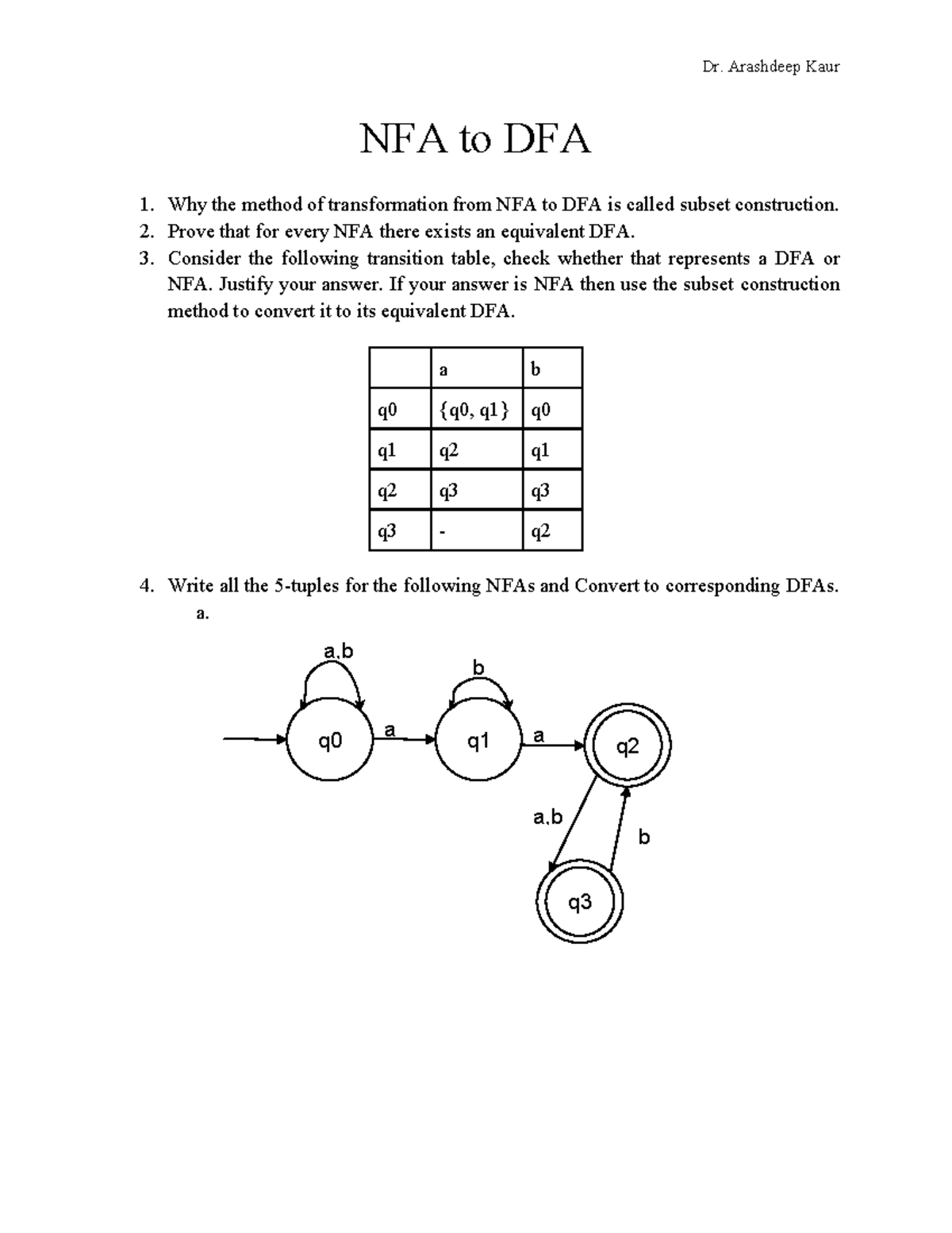
Your task is to convert the NFA shown in problem 4a into an equivalent DFA. Follow the incremental subset construction method we've just discussed.

Identify the start state of the NFA ( $q_{0}$ ). There are no ε-transitions, so the DFA's start state is simply ${q_{0}}$ .
Create a transition table for the DFA, starting with the row for ${q_{0}}$ .
Compute its transitions for inputs a and b.
Each time you discover a new subset (a new DFA state), add a new row for it in the table.
Continue until you have processed all discovered states.
Finally, identify the DFA's accepting states. Which subsets contain the NFA's accepting state, $q_{2}$ ?

Take some time to work through this. You can pause here and draw out the table. Once you're done, you can check your answer. The resulting DFA should have 4 reachable states: ${q_{0}}$ , ${q_{0}, q_{1}}$ , ${q_{0}, q_{2}}$ , and ${q_{0}, q_{1}, q_{3}}$ . The state ${q_{0}, q_{2}}$ is the only accepting state.

Conclusion

In this lesson, we bridged the gap between nondeterministic and deterministic finite automata. You learned that despite their apparent flexibility, NFAs are not more powerful than DFAs. This fundamental result is proven by the subset construction algorithm, which provides a concrete method for converting any NFA into an equivalent DFA.

Here are the key takeaways:

Equivalence of Power: NFAs and DFAs recognize the same class of languages: the regular languages.
Subset Construction: The states of the equivalent DFA correspond to sets of states from the NFA.
The Role of ε-closure: When handling NFAs with ε-transitions, the ε-closure is crucial for correctly defining the DFA's start state and transition function.
State Space Explosion: The conversion can lead to a DFA with an exponential number of states ( $2^{n}$ ) compared to the original NFA ( $n$ ), though in practice, many states are often unreachable.

We have now established a strong foundation with two equivalent models of computation for regular languages. In our next lesson, we will introduce a third, powerful notation: regular expressions. You will learn how to define languages using this algebraic notation and, importantly, how to convert between regular expressions and finite automata, solidifying the deep connection between these three formalisms.

Recommended resources

The Intuition: From Parallel Threads to Deterministic States

The Subset Construction Algorithm

A Practical Walkthrough: Incremental Construction

Practice Your Skills

Conclusion