FCN Encoder-Decoder Architecture for Dense Prediction

The Challenge: From Classification to Dense Prediction

As you know from your background, classic Convolutional Neural Networks (CNNs) like VGG or AlexNet were designed for image classification. They take an image and output a single probability distribution over a set of classes (e.g., "cat," "dog"). This is achieved by progressively downsampling the image through convolutional and pooling layers to extract features, and then feeding these features into one or more fully-connected (FC) layers which collapse all spatial information into a 1D vector for the final prediction.

This architecture presents two major problems for semantic segmentation:

1. Loss of Spatial Information: The FC layers discard the (x, y) location of features, which is precisely what we need for pixel-wise prediction.
2. Fixed Input Size: The fixed number of neurons in the FC layers requires that the input image be of a specific, fixed size (e.g., 224x224 pixels).

To perform dense prediction, we need a network that can process an image of any size and produce an output map of the same spatial dimensions, where each "pixel" in the output corresponds to a class prediction.

The FCN Breakthrough: Convolutionalization

The landmark paper "Fully Convolutional Networks for Semantic Segmentation" proposed an elegant solution to this problem. The core insight was to replace the rigid, space-destroying fully-connected layers with flexible convolutional layers. This process is often called "convolutionalization."

A fully-connected layer can be reinterpreted as a 1x1 convolution where the kernel size is equal to the size of the input feature map. By making this substitution, the network becomes "fully convolutional"—it consists only of convolutional, pooling, and activation layers.

This transformation has two profound consequences:

1. The network can now accept an input image of any size.
2. Instead of a 1D vector, the output is a spatial feature map (a heatmap), where each point corresponds to a classification score for a patch in the original image.

Now that the network produces a spatial output, we have the foundation for an encoder-decoder structure.

The Encoder-Decoder Architecture

The FCN can be conceptually split into two parts: an encoder and a decoder. This is a powerful mental model that applies to many computer vision architectures.

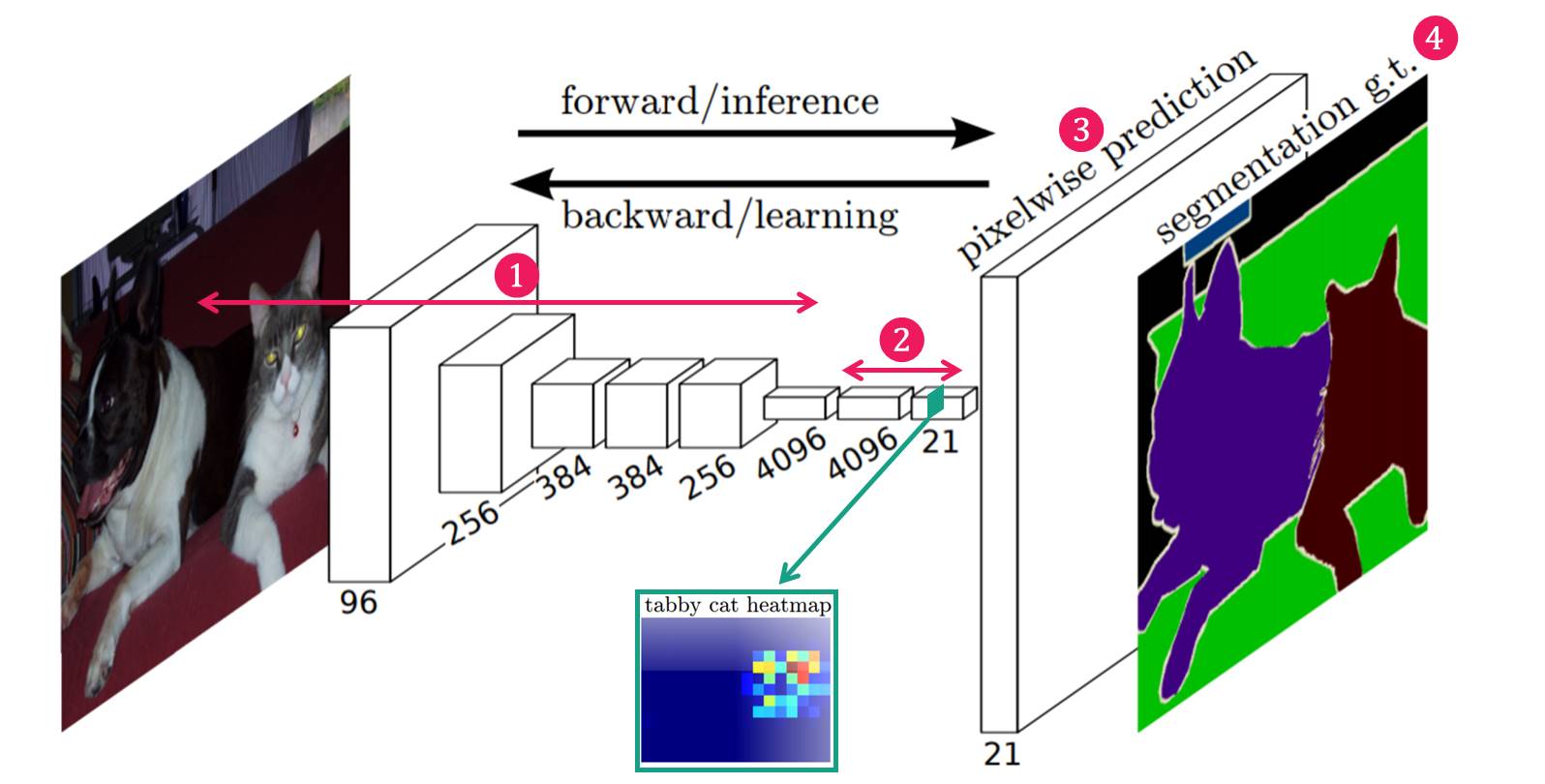
The Encoder: The "What" Pathway

The encoder is typically a pre-trained classification network (like VGG-16) that has been "convolutionalized." Its purpose is to act as a powerful feature extractor. As the image passes through the encoder's layers of convolution and pooling, two things happen:

• The spatial dimensions (height, width) are progressively reduced.
• The feature depth (channels) is progressively increased.

The deeper the layer, the larger its receptive field, and the more semantically abstract the features become. The final output of the encoder is a coarse, low-resolution feature map that encodes what objects are in the image, but has lost the precise information about where they are located.

The Decoder: The "Where" Pathway

The decoder's job is to take the coarse, semantically-rich feature map from the encoder and upsample it back to the original image's resolution to produce a dense, pixel-wise prediction.

But how do we upsample in a way that is learnable? Simple interpolation methods like bilinear upsampling are fixed and not expressive. The FCN paper introduced the idea of using transposed convolution (sometimes called deconvolution) for this task. A transposed convolution is essentially a convolution in reverse: it takes a feature map and increases its spatial resolution. Crucially, like a standard convolution, its kernel weights are learned during training, allowing the network to learn the optimal way to reconstruct spatial detail.

Refining the Output with Skip Connections

Simply taking the final, coarsest layer from the encoder and upsampling it in one go (a variant known as FCN-32s, because the final feature map is downsampled by a factor of 32) produces very rough, blob-like segmentation masks. All the fine-grained spatial detail lost during downsampling cannot be perfectly recovered.

To solve this, the FCN introduced its most important innovation: skip connections.

The idea is to combine deep, coarse, semantic information with shallow, fine-grained, appearance information. The network fuses outputs from different stages of the encoder into the decoder.

This is done by:

1. Taking the output of a deep layer in the decoder.
2. Upsampling it (e.g., by a factor of 2).
3. Taking the output of a shallower layer from the encoder (which has higher resolution).
4. Adding these two feature maps together.
5. Repeating this process until the full resolution is restored.

This allows the network to use the semantic guidance from deep layers to make sense of the scene, while using the fine details from shallow layers to precisely delineate boundaries. This leads to several variants:

• FCN-32s: The baseline model that upsamples the final layer (stride 32) in one step.
• FCN-16s: Fuses the final layer's output with the output from the pool4 layer (stride 16), resulting in a more detailed map.
• FCN-8s: Fuses the FCN-16s output with the output from the pool3 layer (stride 8), yielding even finer results.

By combining convolutionalization, a learnable upsampling path, and multi-scale feature fusion via skip connections, the FCN architecture provides a complete and powerful framework for turning any classification CNN into a dense pixel-wise predictor.

Conclusion

In this lesson, we have deconstructed the Fully Convolutional Network, the model that paved the way for modern semantic segmentation. We saw how it ingeniously solves the limitations of traditional classification networks for dense prediction tasks.

Key Takeaways:

• Encoder-Decoder Structure: FCNs employ an encoder (a downsampling path based on a classification CNN) to extract semantic features, and a decoder (an upsampling path) to reconstruct a full-resolution prediction map.
• Convolutionalization: The key innovation is replacing fixed-size fully-connected layers with 1x1 convolutional layers, allowing the network to accept arbitrary input sizes and produce spatial output maps.
• Learned Upsampling: The decoder uses transposed convolutions to learn how to upsample the coarse feature maps, recovering spatial detail in a data-driven way.
• Skip Connections: To combat the loss of detail from downsampling, FCNs use skip connections to fuse coarse, semantic information from deep layers with fine-grained, appearance information from shallower layers. This combination is critical for producing accurate and detailed segmentation boundaries.

The FCN architecture was revolutionary, but it has its own limitations. The repeated pooling operations in the encoder still result in a significant loss of spatial resolution, which the skip connections can only partially recover. In our next lesson, we will investigate a powerful technique used in models like DeepLabV3 to address this very problem: atrous (or dilated) convolution. This method allows a network to expand its receptive field and capture multi-scale context without aggressive downsampling, preserving crucial spatial information.