Welcome to our next lesson in the Data Structures & Algorithms module. In the previous lesson, we explored recursion, a powerful technique where a function calls itself to solve smaller, self-similar problems. You learned how the call stack manages these calls and implemented the factorial function as a classic example.
Today, we transition from that conceptual foundation to a very practical application: sorting. We'll implement our first sorting algorithm, insertion sort. While this algorithm is iterative, not recursive, the skill of breaking a problem down into smaller, manageable steps is just as crucial. Insertion sort is an intuitive and fundamental algorithm, making it an excellent starting point. It's also highly efficient for small or nearly-sorted datasets, a practical insight that's valuable in real-world software engineering. Our goal is to understand its logic, implement it in Java, and analyze its performance characteristics.
1. The Core Idea: Sorting like Playing Cards
One of the best ways to understand insertion sort is to think about how you might sort a hand of playing cards. Imagine you're dealt cards one by one. You hold the sorted cards in your hand, and with each new card you receive, you find its correct position within your sorted hand and insert it there.
This is precisely how insertion sort works. It partitions the array into two conceptual parts: a sorted sub-array on the left and an unsorted sub-array on the right. Initially, the sorted sub-array contains only the first element (an array of one is always sorted). The algorithm then iterates through the unsorted part, picking one element at a time and "inserting" it into its correct place in the sorted sub-array.
Insertion Sort – Algorithm, Source Code, Time Complexity
This article from Happy Coders starts with the excellent playing card analogy and then transitions into how the algorithm operates on an array.
Read the first two sections, Example: Sorting Playing Cards and Step 2. This will give you a solid mental model of the algorithm's strategy.
2. A Step-by-Step Walkthrough
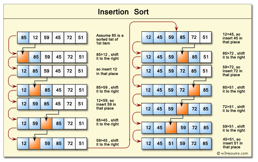
Let's trace the algorithm with a concrete example. Consider the array [85, 12, 59, 45, 72, 51].
- Initial State: The sorted part is
[85]. The unsorted part is[12, 59, 45, 72, 51]. - Pass 1: Pick
12from the unsorted part. Compare it with85. Since12 < 85, shift85one position to the right. Insert12into the now-empty first position. The sorted part is now[12, 85]. - Pass 2: Pick
59. Compare it with85.59 < 85, so we might need to shift. Compare59with12.59 > 12, so we've found the correct spot. Shift85to the right and insert59. The sorted part is[12, 59, 85]. - Pass 3: Pick
45. Compare it with85(shift), then59(shift).45 > 12, so we stop. Insert45. The sorted part is[12, 45, 59, 85].
This process continues until all elements from the unsorted part have been inserted into the sorted part. The following diagram illustrates this entire process clearly.
3. The Shifting Mechanism in Code
A key detail of the implementation isn't swapping elements one by one, but rather shifting larger elements to the right to open up a space for the element we're inserting. This is a more efficient way to move data within the array for this specific algorithm.
Here's how it works in practice:
- Store the current element you want to insert in a temporary variable (e.g.,
currentValue). This frees up its original position in the array. - Work backwards from the position just before
currentValue. - As long as you encounter elements that are greater than
currentValue, copy them one position to their right. - When you either reach the beginning of the array or find an element that is smaller than or equal to
currentValue, you've found the insertion point. - Place
currentValueinto this now-vacant spot.
The following video provides an excellent, detailed visualization of this shifting process, which will make the Java code much easier to understand.
Insertion Sort Algorithm in Java - Full Tutorial With Source
The "Coding with John" channel provides a fantastic visual breakdown of how the shifting works, which is more intuitive than just reading about it.
Watch the segment from this visualization. Pay close attention to how the value being inserted is first copied to a temporary variable, and then the larger elements are shifted one by one to the right before the value is finally placed.
4. Java Implementation
Now that you have a clear picture of the logic, let's look at a clean and well-commented Java implementation. The code directly translates the shifting mechanism we just discussed.
public class InsertionSort {
    public static void sort(int[] arr) {
        // Start from the second element (arr[0] is already 'sorted')
        for (int i = 1; i < arr.length; i++) {
            // The element to be inserted into the sorted portion
            int currentValue = arr[i];

            // j is the index of the last element in the sorted portion
            int j = i - 1;

            // Move elements of arr[0..i-1], that are greater than currentValue,
            // to one position ahead of their current position.
            while (j >= 0 && arr[j] > currentValue) {
                arr[j + 1] = arr[j]; // Shift element to the right
                j--;
            }

            // Place the current value at its correct position
            arr[j + 1] = currentValue;
        }
    }

    public static void main(String[] args) {
        int[] numbers = {85, 12, 59, 45, 72, 51};
        sort(numbers);
        System.out.println(java.util.Arrays.toString(numbers));
        // Output: [12, 45, 51, 59, 72, 85]
    }
}
Let's break down the key parts:
- Outer
forloop:for (int i = 1; i < arr.length; i++). This loop iterates through the unsorted part of the array. We start ati = 1because the first element ati = 0is considered our initial sorted sub-array. currentValue: We savearr[i]before the inner loop starts overwriting array positions.- Inner
whileloop:while (j >= 0 && arr[j] > currentValue). This is the core of the algorithm.j >= 0: Prevents us from going out of bounds at the start of the array.arr[j] > currentValue: This is the comparison that drives the shifting. We continue shifting as long as the element in the sorted part is larger than the value we're trying to insert.
- Insertion:
arr[j + 1] = currentValue;. After thewhileloop finishes,j+1is the correct index forcurrentValue.
5. Performance Analysis
Understanding an algorithm's performance is critical for technical interviews. Let's analyze insertion sort using Big O notation.
| Complexity | Big O Notation |
|---|---|
| Worst case time | |
| Best case time | |
| Average case time | |
| Space |
Source: Adapted from Interview Cake.
Time Complexity
- Worst Case: . This occurs when the array is sorted in reverse order. For each element, we have to shift all the elements in the sorted sub-array. The outer loop runs
ntimes, and the inner loop also runs approximatelyntimes in the worst case, leading to quadratic complexity. - Best Case: . This happens when the array is already sorted. The outer loop still runs
n-1times, but the innerwhileloop's condition (arr[j] > currentValue) is immediately false for every element. So, we only perform a single comparison for each element, resulting in linear time complexity. - Average Case: . For a randomly ordered array, we expect to insert each element somewhere in the middle of the sorted sub-array. This means, on average, the inner loop runs a number of times proportional to
i(the outer loop index), which again leads to quadratic complexity.
Space Complexity
- . Insertion sort is an in-place algorithm. It sorts the array without requiring any significant additional memory. We only use a couple of variables (
currentValue,i,j) to manage the process, regardless of the array's size. This is one of its key strengths.
Insertion Sort – Algorithm, Source Code, Time Complexity
This article provides a more detailed mathematical breakdown of the time complexity and also discusses other important properties like stability.
Read the sections on time complexity to see how the quadratic and linear complexities are derived. Also, read the sections on Other Characteristics and the Summary. Note the point about its stability and its practical use in JDK's Arrays.sort() for small sub-arrays.
Conclusion
In this lesson, you've implemented your first sorting algorithm, insertion sort. It's a foundational algorithm that provides a clear and intuitive way to think about sorting. While its quadratic time complexity makes it unsuitable for very large datasets, its simplicity, O(1) space complexity, and excellent performance on small or nearly-sorted arrays make it an important tool to have in your algorithmic toolkit.
Here are the key takeaways:
- Mechanism: Insertion sort builds a sorted sub-array by picking elements from the unsorted part and inserting them one by one into their correct position.
- Implementation: It uses a nested loop structure, where the inner loop shifts larger elements to the right to make space for the element being inserted.
- Performance: It has a best-case time complexity of , but an average and worst-case of . Its space complexity is .
- Stability: Insertion sort is a stable sort, meaning it preserves the relative order of equal elements.
In our next lesson, we will explore merge sort. This will be a significant step up in efficiency. Merge sort uses a "divide and conquer" strategy, which will bring us back to the recursive thinking you practiced in the previous lesson. You'll see how breaking a problem into halves recursively can lead to a much faster sorting algorithm.