Real-time Spectrograms with FFT

1. Beyond the Fourier Transform: Why We Need the Spectrogram

From your studies, you know the Fourier Transform is a powerful tool for revealing the frequency components of a signal. However, when applied to an entire audio recording, it has a significant limitation: it tells you what frequencies were present, but it gives you no information about when they occurred. An entire symphony and a version of that symphony with all its notes randomly shuffled would have the exact same overall frequency spectrum.

For signals like audio, where the frequency content is constantly changing, we need a tool that provides both time and frequency information. This tool is the spectrogram.

The technique described in the video, often called the Gabor transform when a Gaussian window is used, is a specific instance of a more general method known as the Short-Time Fourier Transform (STFT). This is the mathematical engine we will use to build our spectrogram.

2. The Engine: The Short-Time Fourier Transform (STFT)

The STFT is the formal name for the process of analyzing a long signal by breaking it into shorter, overlapping segments and computing the Fourier Transform on each. This is precisely what our buffering architecture from the last lesson was designed to do.

The time-frequency uncertainty principle is a fundamental concept in signal processing. You can't simultaneously have perfect resolution in both time and frequency. The choice of window size is always a trade-off:

• Large Window (e.g., 4096 samples): Excellent frequency resolution. You can distinguish between very close frequencies (like two adjacent piano notes). However, you lose temporal precision; any event within that window gets smeared out in time. Good for analyzing steady, tonal sounds.
• Small Window (e.g., 256 samples): Excellent time resolution. You can pinpoint the exact moment a transient event occurs (like a drum hit). However, you have poor frequency resolution; distinct frequencies will be blurred together. Good for analyzing rhythmic or percussive sounds.

3. The Spectrogram Algorithm: Step-by-Step

Let's break down the exact sequence of operations your application will perform each time it processes a new frame of audio from the buffer you built in the last lesson.

The process, as outlined in the "Spectrogram Thread" section of the Audio Spectrogram lab guide (resource LINK), is as follows for each audio frame:

1. Acquire Frame: Obtain a block of $N$ audio samples from your input buffer. This block is already windowed, as per our previous lesson's design. $N$ is your FFT size.

2. Compute FFT: Apply an $N$-point Fast Fourier Transform to this block of data.

   $$X[k]=\sum _{n=0}^{N-1}x[n]w[n]e^{-j2\pi kn/N}$$

   where $x[n]$ is the signal, $w[n]$ is the window function, and $X[k]$ are the complex FFT coefficients.

3. Compute Magnitude: The FFT output $X[k]$ is complex. For visualization, we need its magnitude. For a real-valued input signal $x[n]$, the magnitude spectrum is symmetric. We only need to compute and store the first $N/2+1$ values. The magnitude is calculated as:

   $$|X[k]|=\sqrt{\text{Re}(X[k]{)}^2+\text{Im}(X[k]{)}^2}$$

   A practical note: On resource-constrained systems like a microcontroller, the square root operation is computationally expensive. The "Alpha Max Beta Min Algorithm" described in the Audio Spectrogram resource (LINK) offers an efficient approximation: |X[k]| ≈ max(|Re|, |Im|) + 0.4*min(|Re|, |Im|). This is a valuable trick for embedded applications.

4. Convert to Logarithmic Scale (Decibels): The raw magnitude values can have a massive dynamic range. Human hearing is logarithmic, so it's both conventional and more informative to convert the magnitude to a dB scale.

   $$X_{dB}[k]=20{\log }_{10}\left(\frac{|X[k]|}{\text{ref}}\right)$$

   The reference value ref is often set to 1, or sometimes to the maximum possible value of the FFT output.

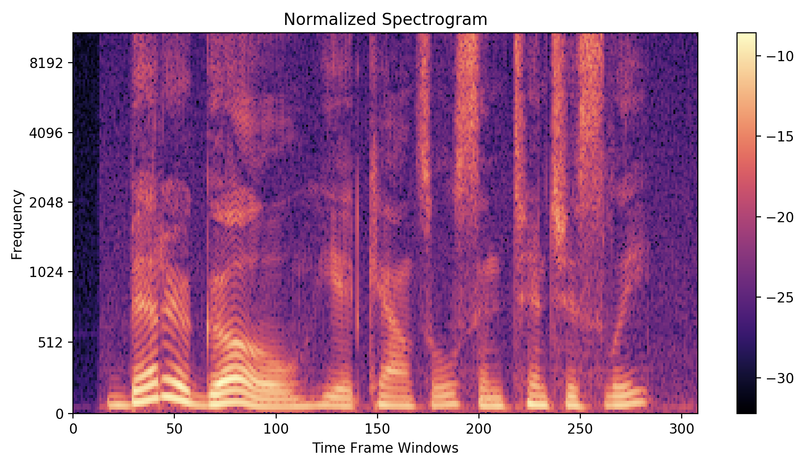
5. Visualize as a Column: This array of $N/2+1$ dB values becomes a single vertical line in our spectrogram image. Each value is mapped to a color based on its level, creating a color-coded representation of the frequency content at that specific moment in time.

4. Implementation and Visualization with Python

While your real-time audio processing core is in C++, the visualization is often best handled by a host computer with more graphical capabilities. A common project architecture involves the C++ application sending the computed spectral data over a serial or network connection to a Python script for display.

Let's simulate this by working directly with an audio file in Python. The scipy library has a powerful function that performs all the STFT steps for us.

Here is a simplified version of the Python code used in the video to generate a spectrogram from an audio file.

import numpy as np
from scipy.io import wavfile
from scipy import signal
import matplotlib.pyplot as plt

# Load the audio file (replace with your file)
# You can often find 'handel.wav' as a standard test file in matplotlib.
# Or use any .wav file you have.
fs, x = wavfile.read('path_to_your_audio.wav') 

# If stereo, take only one channel
if x.ndim > 1:
    x = x[:, 0]

# --- Parameters for STFT ---
# These should match the parameters in your C++ buffering system
window_size = 1024
hop_size = 512 # This is overlap = window_size - hop_size = 512
window_function = 'hann'

# Compute the spectrogram
# f = frequencies, t = times, Sxx = spectrogram values
f, t, Sxx = signal.spectrogram(x, 
                               fs=fs, 
                               window=window_function, 
                               nperseg=window_size, 
                               noverlap=hop_size)

# Plot the spectrogram
plt.figure(figsize=(10, 6))
# Use pcolormesh for plotting. Sxx is in power, so 10*log10 for dB.
# Add a small epsilon to avoid log(0).
plt.pcolormesh(t, f, 10 * np.log10(Sxx + 1e-10), shading='gouraud')

plt.ylabel('Frequency [Hz]')
plt.xlabel('Time [sec]')
plt.title('Spectrogram')
plt.colorbar(label='Intensity [dB]')
plt.ylim(0, 8000) # Limit frequency range to typical human hearing
plt.show()

This Python script is the perfect counterpart to your C++ engine. Your C++ code would calculate the FFT for each frame and could send the resulting magnitude vector (Sxx for one time slice) to a Python script that then plots it as a new column in a continuously updating pcolormesh plot.

Conclusion

You have now connected your real-time buffering framework to the powerful analysis capabilities of the FFT. You understand the theory behind the spectrogram as a time-frequency representation of a signal and have seen how to compute and visualize it.

Key Takeaways:

• The spectrogram visualizes how a signal's frequency content evolves over time, overcoming the limitations of the standard Fourier Transform for non-stationary signals.
• The underlying algorithm is the Short-Time Fourier Transform (STFT), which involves computing FFTs on a sequence of overlapping, windowed data frames.
• There is a fundamental time-frequency uncertainty trade-off controlled by the window size: large windows give good frequency resolution, while small windows give good time resolution.
• The computation for each frame involves: FFT -> Magnitude -> Logarithmic (dB) scaling.
• Python libraries like scipy.signal.spectrogram provide a high-level way to perform this analysis, which is ideal for creating a visualization front-end for your real-time system.

Preview of the Next Lesson:

Now that you can see the spectrum of your audio in real time, the next logical step is to change it. In the next lesson, you will learn to design a lowpass or bandpass filter (IIR or FIR) to meet a specific audio frequency cutoff specification. This will be your first tool for actively shaping the sound of your audio stream.