Deriving the Sampling Theorem from Impulse Sampling

1. A Mathematical Model for Sampling

To analyze sampling using the continuous-time Fourier transform (CTFT), we need a mathematical model that exists in the continuous-time domain. While a real-world sampler creates a discrete sequence of numbers, $x[n]$, our analytical tool will be impulse sampling.

In this model, we represent the sampled signal, which we'll call $x_s(t)$, as the original continuous-time signal, $x(t)$, multiplied by an infinite train of Dirac delta functions, $p(t)$. This impulse train is defined as:
$p(t)={\sum }_{n=-\infty }^{\infty }\delta (t-n{T}_s)$
where $T_s$ is the sampling period.

The resulting impulse-sampled signal is:
$x_s(t)=x(t)\cdot p(t)=x(t){\sum }_{n=-\infty }^{\infty }\delta (t-n{T}_s)$
Using the sifting property of the delta function, this simplifies to:
$x_s(t)={\sum }_{n=-\infty }^{\infty }x(n{T}_s)\delta (t-n{T}_s)$
This gives us a continuous-time signal that is zero everywhere except at the sampling instants $t=n{T}_s$, where it consists of impulses whose "areas" are equal to the sample values $x(n{T}_s)$.

2. The Spectrum of a Sampled Signal

Now for the crucial question: What does the spectrum of our impulse-sampled signal, $X_s(\omega )$, look like?

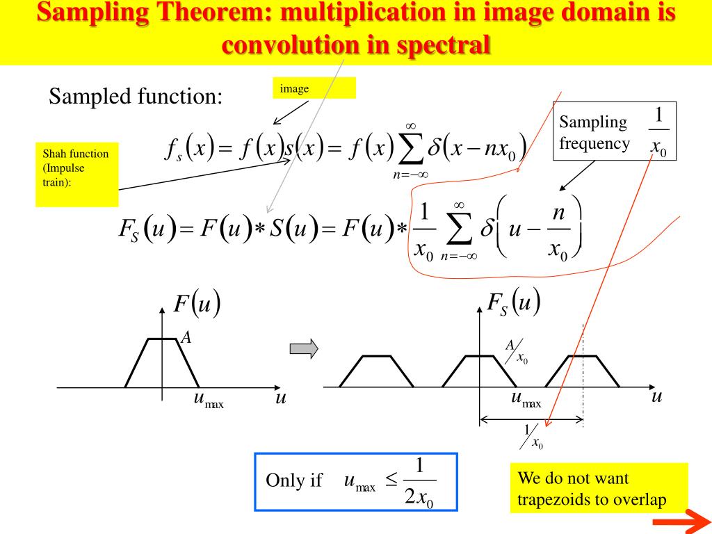
From your background in signal processing, you know that multiplication in the time domain corresponds to convolution in the frequency domain. Therefore:
$X_s(\omega )=\mathcal{F}\{x(t)\cdot p(t)\}=\frac{1}{2\pi }[X(\omega )\ast P(\omega )]$
To solve this, we need the Fourier transform of the impulse train, $P(\omega )$. Since $p(t)$ is a periodic function, its Fourier transform is not a continuous function but another impulse train in the frequency domain. The derivation relies on the Fourier series representation of $p(t)$.

After working through the derivation, you arrive at the central result of sampling analysis:
$X_s(\omega )=\frac{1}{T_s}{\sum }_{k=-\infty }^{\infty }X(\omega -k{\omega }_s)$
where ${\omega }_s=2\pi /T_s$ is the sampling frequency in radians per second.

This equation is profound. It tells us that the spectrum of the sampled signal is a summation of infinitely many copies of the original signal's spectrum, $X(\omega )$. These copies are scaled by $1/T_s$ and shifted in frequency by integer multiples of the sampling frequency ${\omega }_s$.

3. Deriving the Nyquist Criterion

Now we can see the sampling theorem emerge directly from this spectral analysis. Let's assume our original signal $x(t)$ is band-limited, meaning its spectrum $X(\omega )$ is zero for all frequencies above some maximum frequency, ${\omega }_m$. That is, $X(\omega )=0$ for $|\omega |>{\omega }_m$.

The video below provides a clear, graphical derivation of the sampling condition based on the spectral replication we just proved.

As the video demonstrates, to be able to perfectly recover the original spectrum $X(\omega )$ from the sampled spectrum $X_s(\omega )$, the replicated copies must not overlap. We can simply filter out all the copies using an ideal low-pass filter to isolate the original centered at $\omega =0$.

Let's look at the boundary between the original spectrum and the first replica (for $k=1$):

• The highest frequency of the original spectrum is at ${\omega }_m$.
• The first replica is centered at ${\omega }_s$, so its lowest frequency is at ${\omega }_s-{\omega }_m$.

For these two not to overlap, we require:
${\omega }_s-{\omega }_m\ge {\omega }_m$
Rearranging this gives the celebrated Nyquist Criterion:
${\omega }_s\ge 2{\omega }_m$
In terms of cyclical frequency $f$ (in Hz), where $\omega =2\pi f$, this is $f_s\ge 2f_m$. This confirms Shannon's statement: a band-limited signal can be perfectly reconstructed if the sampling rate is at least twice its highest frequency. The critical rate $2f_m$ is what Shannon called the Nyquist rate.

4. The Formal Proof and Reconstruction

We have now derived the theorem intuitively. For completeness, let's look at the formal mathematical proof, which also introduces the ideal reconstruction filter.

The reading shows that the process of ideal reconstruction involves filtering $x_s(t)$ with an ideal low-pass filter whose impulse response is a sinc function. This confirms that if the Nyquist criterion is met, the original continuous-time signal is recoverable in its entirety from the samples.

Conclusion

In this lesson, we have constructed the mathematical foundation of the sampling theorem. By modeling sampling as multiplication by an impulse train, we've seen how this seemingly simple time-domain operation leads to a fundamental and beautiful result in the frequency domain.

Key Takeaways:

• Impulse Sampling Model: Multiplying a signal $x(t)$ by an impulse train $p(t)$ creates a mathematically tractable model for sampling, $x_s(t)$.
• Spectral Replication: The Fourier transform of the sampled signal, $X_s(\omega )$, is a periodic repetition of the original signal's spectrum, $X(\omega )$, scaled and shifted by multiples of the sampling frequency ${\omega }_s$.
  $X_s(\omega )=\frac{1}{T_s}{\sum }_{k=-\infty }^{\infty }X(\omega -k{\omega }_s)$
• The Nyquist Criterion: To enable perfect reconstruction of a signal band-limited to ${\omega }_m$, the spectral replicas must not overlap. This leads to the condition ${\omega }_s\ge 2{\omega }_m$.
• Ideal Reconstruction: If the Nyquist criterion is met, the original signal can be perfectly recovered by passing the impulse-sampled signal through an ideal low-pass filter.

Preview of the Next Lesson:
We have established the condition for perfect sampling. But what happens if we break the rule? In the next lesson, we will analyze the phenomenon of aliasing mathematically and derive the conditions for alias-free signal reconstruction. We will investigate exactly what happens when the spectral replicas overlap and how higher frequencies masquerade as lower frequencies, a critical concept for any practical digital system.