ROC Curves and AUC Score for Model Comparison

1. Beyond Accuracy: The Need for a Better Metric

Most classification models, like Logistic Regression, don't just predict a class (e.g., 'Yes' or 'No'). They output a probability of belonging to the positive class. We typically use a threshold of 0.5 to convert this probability into a final decision: if the probability is > 0.5, we predict 'Yes'; otherwise, we predict 'No'.

But what if 0.5 isn't the best threshold for our problem? In medical screening, we might want to lower the threshold to catch as many true positive cases as possible, even if it means more false alarms. In spam filtering, we might raise the threshold to be very sure something is spam before moving it, avoiding the high cost of a false positive (a real email ending up in the spam folder).

The Receiver Operating Characteristic (ROC) curve is a tool that helps us see how a model performs across all possible thresholds.

To understand how an ROC curve is constructed, we need to first grasp its two key components: the True Positive Rate and the False Positive Rate.

• True Positive Rate (TPR): Of all the actual positive instances, what fraction did we correctly identify? TPR = TP / (TP + FN)
• False Positive Rate (FPR): Of all the actual negative instances, what fraction did we incorrectly identify as positive? FPR = FP / (FP + TN)

The ROC curve plots TPR (y-axis) against FPR (x-axis) for every possible threshold.

2. Building the ROC Curve: An Intuitive Walkthrough

How do we get from a set of probabilities to a full curve? The best way to understand this is to build one step-by-step.

The following video from StatQuest provides an exceptionally clear, intuitive explanation of this process. It shows how changing the classification threshold on a logistic regression model generates different pairs of TPR and FPR values, which then become points on our ROC curve.

This step-by-step process is what scikit-learn does for us automatically, but seeing it done manually is key to truly understanding what the curve represents.

3. Interpreting the Curve and the AUC Score

Now that you've seen how an ROC curve is made, how do we interpret it?

• A Perfect Classifier: Would have a TPR of 1 and an FPR of 0. This corresponds to the top-left corner (0,1) of the plot. The closer an ROC curve hugs this corner, the better the model.
• A Random Classifier: Is represented by the diagonal line from (0,0) to (1,1). If your model's curve is on or below this line, it's no better than random guessing.

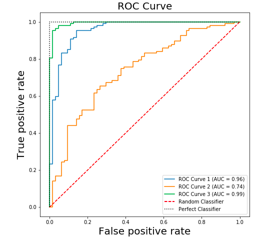
While the curve is a great visual tool, it's often useful to summarize its performance into a single number. This is where the Area Under the Curve (AUC) comes in.

The AUC score is the area under the ROC curve. It is a value between 0 and 1.

• AUC = 1.0: A perfect classifier.
• AUC = 0.5: A classifier that is no better than random chance.
• AUC > 0.5: A classifier that has some discriminative power.

Let's return to the StatQuest video to see how AUC helps us compare models.

The model with the higher AUC score is generally the better classifier.

4. Plotting ROC and Calculating AUC in Python

Let's get practical. You've already used scikit-learn to train models; now we'll use it to evaluate them with ROC and AUC. The process is straightforward:

1. Train your classification models as usual.
2. Use model.predict_proba(X_test) to get the predicted probabilities for the test set. This is crucial! The ROC functions need probabilities, not the final class predictions from model.predict().
3. Use sklearn.metrics.roc_auc_score() to calculate the AUC.
4. Use sklearn.metrics.roc_curve() to get the FPR and TPR values needed for plotting.
5. Use matplotlib to plot the curve.

The following guide provides clear, step-by-step Python code for doing exactly this, including a great example of comparing multiple models on the same plot.

Here is a self-contained example you can run. We will train a Logistic Regression and a K-Nearest Neighbors model (both of which you're familiar with) and compare them.

import pandas as pd
import matplotlib.pyplot as plt
from sklearn.model_selection import train_test_split
from sklearn.datasets import make_classification
from sklearn.linear_model import LogisticRegression
from sklearn.neighbors import KNeighborsClassifier
from sklearn.metrics import roc_curve, roc_auc_score




# 1. Generate synthetic data
X, y = make_classification(n_samples=1000, n_classes=2, random_state=42)
X_train, X_test, y_train, y_test = train_test_split(X, y, test_size=0.3, random_state=42)




# 2. Train models
log_reg = LogisticRegression().fit(X_train, y_train)
knn = KNeighborsClassifier(n_neighbors=5).fit(X_train, y_train)




# 3. Get prediction probabilities for the positive class (class 1)
log_reg_probs = log_reg.predict_proba(X_test)[:, 1]
knn_probs = knn.predict_proba(X_test)[:, 1]




# 4. Calculate AUC scores
log_reg_auc = roc_auc_score(y_test, log_reg_probs)
knn_auc = roc_auc_score(y_test, knn_probs)
print(f"Logistic Regression AUC: {log_reg_auc:.4f}")
print(f"KNN AUC: {knn_auc:.4f}")




# 5. Calculate ROC curve values
fpr_log, tpr_log, _ = roc_curve(y_test, log_reg_probs)
fpr_knn, tpr_knn, _ = roc_curve(y_test, knn_probs)




# 6. Plot the ROC curves
plt.figure(figsize=(8, 6))
plt.plot(fpr_log, tpr_log, label=f'Logistic Regression (AUC = {log_reg_auc:.2f})')
plt.plot(fpr_knn, tpr_knn, label=f'KNN (AUC = {knn_auc:.2f})')
plt.plot([0, 1], [0, 1], 'k--', label='Random Classifier') # Diagonal line

plt.xlabel('False Positive Rate')
plt.ylabel('True Positive Rate')
plt.title('ROC Curve Comparison')
plt.legend(loc='lower right')
plt.show()

This code produces a plot that allows for a direct visual and numerical comparison of the two models. The model with the higher AUC and the curve closer to the top-left is superior.

Conclusion

Congratulations! You can now evaluate and compare classification models using one of the most standard and insightful techniques in machine learning. This method provides a much more nuanced view of performance than accuracy alone.

Key Takeaways:

• An ROC curve visualizes a classifier's performance by plotting the True Positive Rate (TPR) against the False Positive Rate (FPR) across all possible classification thresholds.
• A model whose curve is closer to the top-left corner is better. The diagonal line represents a random-chance model.
• The Area Under the Curve (AUC) summarizes the ROC curve into a single value from 0.5 (random) to 1.0 (perfect).
• To compare models, you can plot their ROC curves on the same axes and compare their AUC scores. The model with the higher AUC is generally better.
• In Python, you must use predict_proba() to get the probabilities required by roc_curve() and roc_auc_score().

Preview of the next lesson:
Plotting an ROC curve on a single test set is a great step. However, the performance can vary depending on how the data was split. To get a more reliable and robust estimate of model performance, we should combine our evaluation with cross-validation. In the next lesson, we will learn how to systematically compare multiple models using cross-validated metrics, giving you the confidence to select a final model that is expected to generalize well to new, unseen data.