XGBoost: Beyond Gradient Boosting

1. What Makes XGBoost "Extreme"?

While XGBoost follows the same sequential, error-correcting logic as standard gradient boosting, it incorporates numerous enhancements that make it faster, more accurate, and more robust against overfitting. These improvements are why it has a reputation for winning machine learning competitions.

This table provides a high-level comparison between standard Gradient Boosting (like scikit-learn's implementation) and XGBoost.

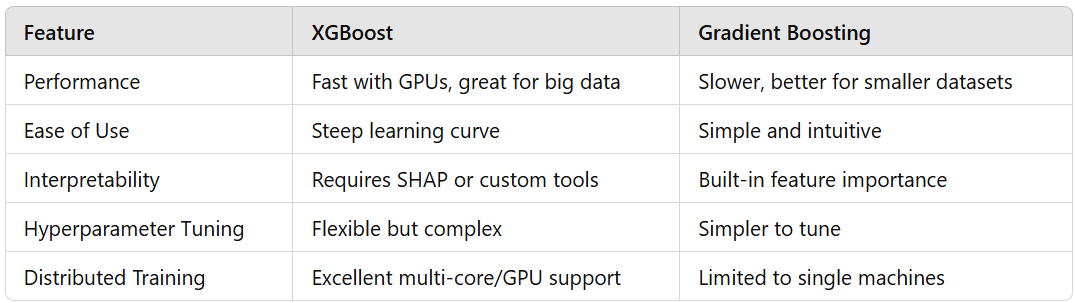
Let's break down the main advantages that make XGBoost so powerful.

To summarize and expand on the video, here are the core advantages of XGBoost over standard gradient boosting:

1. Superior Performance and Speed: XGBoost is written in C++ and is highly optimized for performance. It can train models significantly faster, often by an order of magnitude, by using techniques like parallel processing (utilizing all your CPU cores to build trees) and optimized data structures.

2. Advanced Regularization: This is a key factor in its high accuracy. Standard gradient boosting can be prone to overfitting if not carefully tuned. XGBoost includes more advanced regularization techniques built directly into its objective function:

   • L1 (Alpha) and L2 (Lambda) regularization on the leaf weights, similar to what you've seen in Ridge and Lasso regression. This penalizes large weights and helps create a simpler, more generalizable model.
   • Gamma (min_split_loss) regularization on the number of tree nodes, which prunes trees by penalizing splits that don't provide sufficient loss reduction.

3. Smarter Optimization: While standard gradient boosting uses only the first derivative (the gradient or "slope") of the loss function to correct errors, XGBoost uses both the first and second derivatives (the gradient and the Hessian, which measures "curvature"). This provides more information about the loss function, allowing the algorithm to take more direct and accurate steps towards the optimal solution, often resulting in faster convergence and a better final model.

4. Built-in Feature Handling:

   • Sparsity-Aware Algorithm: XGBoost can automatically handle missing values (NaN). It learns the best direction to send data points with missing values at each node, eliminating the need for you to perform imputation beforehand.
   • Built-in Cross-Validation: XGBoost has its own internal cross-validation function that can be run at each iteration of the boosting process.

For a clear textual summary of these benefits, the following reading is excellent.

2. Training an XGBoost Model in Python

Now let's get practical. One of the best features of the xgboost library is its scikit-learn compatible API. This means you can use it just like any other scikit-learn model, making it easy to integrate into the workflows you've already learned.

First, you'll need to install the library if you haven't already. You can do this by running the following command in your terminal or a code cell:

pip install xgboost

The primary class we'll use is xgboost.XGBClassifier. You'll notice many of its hyperparameters are familiar from GradientBoostingClassifier, such as n_estimators, learning_rate, and max_depth.

The following resource provides a simple, complete example of training an XGBClassifier.

Here is the core of that example, distilled into its essential parts:

# 1. Import necessary libraries
import xgboost as xgb
from sklearn.datasets import load_iris
from sklearn.model_selection import train_test_split
from sklearn.metrics import accuracy_score




# 2. Load and split the data
X, y = load_iris(return_X_y=True)
X_train, X_test, y_train, y_test = train_test_split(X, y, test_size=0.2, random_state=42)




# 3. Initialize an XGBoost classifier
# We set use_label_encoder=False and eval_metric='mlogloss' to use the latest standards
# and avoid potential deprecation warnings.
model = xgb.XGBClassifier(
    objective='multi:softprob', # Specify the objective for multi-class classification
    use_label_encoder=False, 
    eval_metric='mlogloss',
    random_state=42
)




# 4. Train the model
model.fit(X_train, y_train)




# 5. Make predictions and evaluate
y_pred = model.predict(X_test)
accuracy = accuracy_score(y_test, y_pred)
print(f"Accuracy: {accuracy * 100:.2f}%")

Integrating XGBoost into a Pipeline

Just like with the GradientBoostingClassifier, the best practice is to include your XGBClassifier as the final step in a scikit-learn Pipeline. This ensures that any preprocessing steps are applied consistently and helps prevent data leakage.

Let's imagine our Iris dataset needed preprocessing. Here’s how you would structure the workflow:

import xgboost as xgb
from sklearn.pipeline import Pipeline
from sklearn.preprocessing import StandardScaler
from sklearn.datasets import load_iris
from sklearn.model_selection import train_test_split
from sklearn.metrics import accuracy_score




# Load and split data
X, y = load_iris(return_X_y=True)
X_train, X_test, y_train, y_test = train_test_split(X, y, test_size=0.2, random_state=42)




# Create a pipeline
# Step 1: Scale the data (though not strictly necessary for tree models, it's good practice for many algorithms)
# Step 2: Fit the XGBoost classifier
pipeline = Pipeline([
    ('scaler', StandardScaler()),
    ('xgb', xgb.XGBClassifier(
        objective='multi:softprob',
        use_label_encoder=False,
        eval_metric='mlogloss',
        random_state=42
    ))
])




# Fit the entire pipeline
pipeline.fit(X_train, y_train)




# Predict using the pipeline
y_pred = pipeline.predict(X_test)
accuracy = accuracy_score(y_test, y_pred)
print(f"Pipeline Accuracy: {accuracy * 100:.2f}%")

This structure should feel very familiar and demonstrates how easily XGBoost fits into a robust, production-ready workflow.

3. A Hands-on Comparison

To solidify your understanding, let's do a quick diagnostic exercise. We'll train both a GradientBoostingClassifier and an XGBClassifier on the same data and compare their training time and accuracy.

Here's a code snippet you can run in a notebook. We'll use scikit-learn's make_classification to create a slightly more challenging synthetic dataset.

import time
from sklearn.datasets import make_classification
from sklearn.model_selection import train_test_split
from sklearn.metrics import accuracy_score
from sklearn.ensemble import GradientBoostingClassifier
import xgboost as xgb




# 1. Create a synthetic dataset
X, y = make_classification(
    n_samples=10000, 
    n_features=50, 
    n_informative=20, 
    n_redundant=10, 
    random_state=42
)
X_train, X_test, y_train, y_test = train_test_split(X, y, test_size=0.2, random_state=42)




# 2. Train and time scikit-learn's GradientBoostingClassifier
print("Training GradientBoostingClassifier...")
gb_model = GradientBoostingClassifier(n_estimators=100, learning_rate=0.1, max_depth=3, random_state=42)
start_time = time.time()
gb_model.fit(X_train, y_train)
gb_time = time.time() - start_time
gb_pred = gb_model.predict(X_test)
gb_accuracy = accuracy_score(y_test, gb_pred)

print(f"Time taken: {gb_time:.4f} seconds")
print(f"Accuracy: {gb_accuracy:.4f}\n")




# 3. Train and time XGBoost
print("Training XGBClassifier...")
xgb_model = xgb.XGBClassifier(n_estimators=100, learning_rate=0.1, max_depth=3, random_state=42, use_label_encoder=False, eval_metric='logloss')
start_time = time.time()
xgb_model.fit(X_train, y_train)
xgb_time = time.time() - start_time
xgb_pred = xgb_model.predict(X_test)
xgb_accuracy = accuracy_score(y_test, xgb_pred)

print(f"Time taken: {xgb_time:.4f} seconds")
print(f"Accuracy: {xgb_accuracy:.4f}\n")




# 4. Compare results
print("--- Comparison ---")
print(f"XGBoost was {gb_time / xgb_time:.2f}x faster than GradientBoostingClassifier.")
print(f"Accuracy difference (XGB - GB): {xgb_accuracy - gb_accuracy:.4f}")

When you run this code, you will likely observe that XGBoost trains significantly faster while achieving comparable or even slightly better accuracy. This is a direct, practical demonstration of its performance advantage.

Conclusion

Congratulations! You've now added XGBoost to your ensemble methods toolkit. You've seen that while it shares its DNA with standard gradient boosting, its "extreme" optimizations provide significant advantages in the real world.

Key Takeaways:

• XGBoost is a highly optimized implementation of gradient boosting known for its speed, accuracy, and robustness.
• Its main advantages come from parallel processing, more advanced regularization (L1, L2, gamma), smarter optimization using second-order gradients, and built-in handling for missing values.
• The xgboost Python library provides a scikit-learn compatible API (XGBClassifier, XGBRegressor), making it easy to integrate into Pipeline workflows you are already familiar with.

Preview of the next lesson:
Now that you have several powerful models in your arsenal (Decision Trees, Random Forests, Gradient Boosting, XGBoost), our next lesson will focus on a crucial skill: systematically comparing their performance. We'll establish a framework for evaluating whether a complex ensemble model truly offers an advantage over a simpler baseline for a given problem.