Hierarchical Clustering and Dendrogram Interpretation

1. Understanding Hierarchical Clustering

Hierarchical clustering creates a set of nested clusters that are organized as a tree. There are two main strategies for this:

1. Agglomerative (Bottom-Up): This is the most common approach. We start by treating each data point as its own cluster. Then, at each step, we merge the two closest clusters until only one cluster (containing all data points) remains.
2. Divisive (Top-Down): This method is the opposite. We start with all data points in a single cluster and, at each step, split a cluster until every data point is in its own cluster.

Because the agglomerative approach is more widely used and computationally more efficient, we will focus on it for this lesson.

To get a clear conceptual overview of these ideas, please watch the following short video.

2. The Core Choices: Distance Metric and Linkage Criterion

The agglomerative process sounds straightforward: "merge the two closest clusters." But how do we define "closest"? This requires two key decisions:

1. Distance Metric: This defines how we measure the distance between two individual data points. You're already familiar with the most common one, Euclidean distance (the straight-line distance). Other options, like Manhattan or Cosine distance, exist for different use cases.
2. Linkage Criterion: This defines how we measure the distance between two clusters, which may contain multiple points. This choice significantly affects the final structure of the hierarchy.

The four most common linkage criteria are:

• Single Linkage: The distance between two clusters is the distance between the closest pair of points (one from each cluster). This method is good at identifying non-elliptical shapes and outliers, but can sometimes produce long, stringy clusters (a phenomenon called "chaining").
• Complete Linkage: The distance is defined by the farthest pair of points. This method tends to produce more compact, spherical clusters.
• Average Linkage: The distance is the average of all pairwise distances between points in the two clusters. It's a compromise between single and complete linkage.
• Ward's Linkage: This is a popular and often effective default choice. It merges the two clusters that result in the minimum increase in the total within-cluster variance. In simpler terms, it tries to find the most compact, spherical clusters, similar to K-Means.

To solidify these concepts and get some practical advice on choosing them, the next video is very helpful.

The image below visually demonstrates how different linkage criteria produce very different cluster hierarchies (dendrograms) even on the same data.

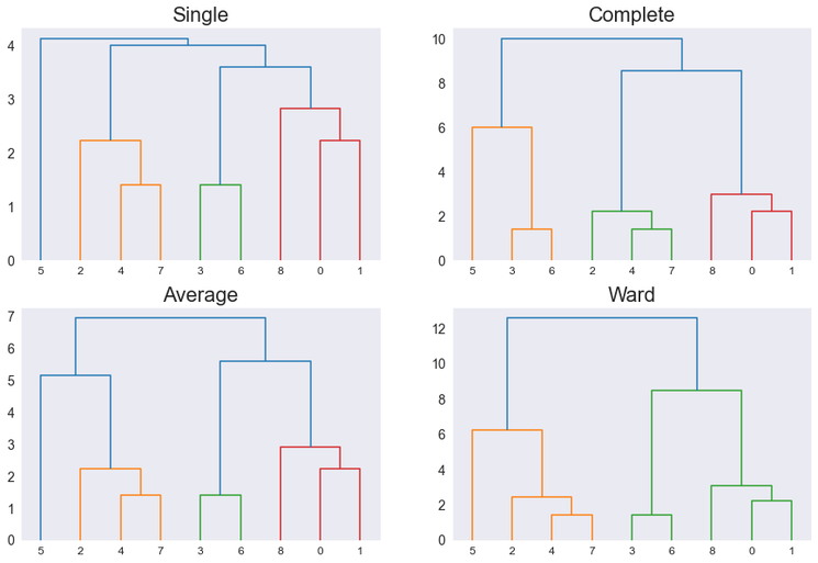
3. Interpreting the Dendrogram

The result of a hierarchical clustering algorithm is a dendrogram, a tree diagram that visually represents the entire hierarchy of merges. This is the key tool for interpreting your results.

Let's break down how to read one:

• The y-axis represents the distance or dissimilarity. The height of the horizontal line connecting two clusters shows the distance at which they were merged.
• The x-axis lists the individual data points.
• By following the lines upwards, you can trace the history of merges, from individual points to the final single cluster.

The most important use of a dendrogram is to help you decide on the number of clusters. You do this by setting a distance threshold—essentially drawing a horizontal line across the dendrogram.

The rule of thumb is to make a cut where there is a large vertical distance with no merges. This long vertical line signifies that two very dissimilar clusters were merged, and it's often a good point to stop.

The following video provides an excellent walkthrough of reading and interpreting a dendrogram to find clusters.

4. Hierarchical Clustering in Python with SciPy

Now let's move to the practical application. While scikit-learn has an implementation, the scipy library is often preferred for hierarchical clustering because its functions map directly to the concepts we've learned and provide the tools to easily generate dendrograms.

The main functions we'll use are:

• scipy.cluster.hierarchy.linkage(): Takes your data and performs the hierarchical clustering using your chosen method (e.g., 'ward') and metric (e.g., 'euclidean'). It returns a linkage matrix, which encodes the merge history.
• scipy.cluster.hierarchy.dendrogram(): Takes the linkage matrix and plots the corresponding dendrogram.
• scipy.cluster.hierarchy.fcluster(): Takes the linkage matrix and a criterion (like a distance threshold or a target number of clusters) and returns the cluster labels for each data point.

The following tutorial provides a superb, step-by-step guide to implementing this entire workflow.

By following this tutorial, you will have completed the full cycle: performing the clustering, interpreting the dendrogram to choose a cluster count, and extracting those clusters for further analysis.

Conclusion

Congratulations! You've just learned one of the most fundamental and intuitive clustering methods. Unlike K-Means, hierarchical clustering provides a rich, visual output that allows you to explore relationships at multiple scales without committing to a number of clusters beforehand.

Key Takeaways:

• Hierarchical clustering builds a nested tree of clusters, most commonly using an agglomerative (bottom-up) approach.
• The algorithm requires two key choices: a distance metric (like Euclidean) and a linkage criterion (like Ward, complete, or single).
• The dendrogram is the primary output, visualizing the entire merge history. The height of merges represents the dissimilarity between the clusters.
• You can determine the number of clusters by finding a large vertical gap in the dendrogram and "cutting" the tree at that height.
• The scipy.cluster.hierarchy module provides powerful and intuitive tools (linkage, dendrogram, fcluster) to perform and interpret hierarchical clustering.

Preview of the next lesson:
So far in this module, we've focused on finding groups within our data. In the next lesson, we will pivot to a different unsupervised learning task: dimensionality reduction. We'll learn about Principal Component Analysis (PCA), a powerful technique for reducing the number of features in a dataset while retaining most of the important information. This is essential for visualization, noise reduction, and improving the performance of other machine learning algorithms.