Spatial Data Types for Public Health

The Two Families of Spatial Data

In epidemiology, you are accustomed to collecting data about individuals or populations—their health status, exposures, and demographics. Spatial analysis adds a new, powerful dimension: location. It's not just what is happening, but where it is happening. To represent location information on a computer, we use specialized formats. All spatial data can be categorized into two main families: vector and raster.

Let's begin by looking at a diagram that illustrates this fundamental difference.

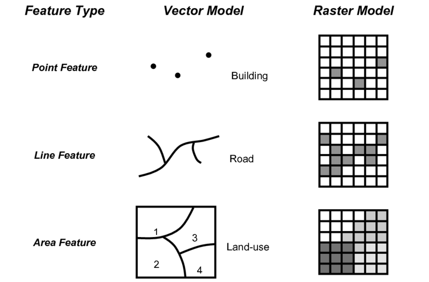
As you can see, the vector model represents the world using distinct, geometric shapes, while the raster model uses a continuous grid of cells, much like a digital photograph. Let's explore each of these in more detail.

Vector Data: Representing Discrete Objects

Vector data is used to represent features that have clear, discrete boundaries. Think of it as drawing specific objects on a map. These objects are built from three basic geometric types:

1. Points: A single pair of coordinates (latitude and longitude) that represents a specific location. In public health, points are incredibly useful for mapping:

   • The homes of patients in a disease outbreak investigation.
   • The locations of healthcare facilities, like hospitals or clinics.
   • Sites where environmental samples were taken (e.g., water quality tests).

2. Lines: A sequence of connected points. Lines have a length and are used to represent linear features. Health-related examples include:

   • Road networks, which are essential for analyzing travel time to hospitals.
   • Rivers, which might be a source of exposure to waterborne diseases or act as a barrier to movement.
   • The routes traveled by mobile health units or contact tracing teams.

3. Polygons: A series of connected lines that form a closed shape. Polygons have a perimeter and an area, making them ideal for representing boundaries. In spatial epidemiology, polygons are fundamental for:

   • Administrative boundaries, such as states, counties, or census tracts, which are used to aggregate and map health statistics like disease rates.
   • Hospital catchment areas or health service districts.
   • The footprint of a park, which could be analyzed for its impact on community health.

The Power of Attributes

A crucial feature of vector data is that each point, line, or polygon is linked to a row in a data table called an attribute table. This table holds all the non-spatial information about that feature. For example, a point representing a hospital might have attributes for its name, number of beds, and types of services offered. A polygon representing a county could have attributes for its total population, the number of disease cases, and demographic information. This ability to link rich, descriptive data to geographic features is what makes spatial analysis so powerful.

To see these concepts explained visually, the following video provides a clear overview of vector data and the importance of attribute tables.

Raster Data: Representing Continuous Surfaces

While vector data excels at representing discrete objects, many phenomena in our world don't have sharp edges. Think about air temperature, elevation, or population density. These things exist everywhere across a landscape, changing gradually from one place to another. To represent this kind of continuous data, we use the raster model.

A raster is essentially a grid of cells, or pixels, covering a specific area. Each pixel in the grid has a specific value that represents the characteristic being measured at that location.

Common examples of raster data in public health include:

• Environmental Data: Satellite imagery can be processed to create rasters showing continuous surfaces of air pollution (e.g., PM2.5 levels), land surface temperature, or vegetation cover, all of which can be linked to health outcomes.
• Population Density: Organizations like WorldPop provide global raster datasets that estimate the number of people living in each 100x100 meter grid cell, which is invaluable for calculating disease rates where precise census data is unavailable.
• Elevation Models: A raster where each pixel's value is its height above sea level. This can be used to model the habitat of disease vectors (like mosquitoes) or to understand physical barriers to healthcare access.

The video you watched earlier also has a great segment on raster data. Let's watch it now to solidify your understanding.

Reinforcing the Concepts

To ensure these definitions are clear, let's turn to a couple of short readings that directly address these concepts in a public health context.

First, this guide was developed for a QGIS workshop for public health professionals. It provides concise, relevant definitions and examples.

Next, this chapter from "The Epidemiologist R Handbook" presents the same concepts, reinforcing that this knowledge is platform-independent—it is just as crucial for programming in R as it is for using point-and-click software like QGIS.

Bringing It All Together

In practice, you will rarely use just one data type. Most spatial analyses involve combining vector and raster data. For example, you might overlay vector points representing patient locations onto a raster surface of air pollution to estimate each patient's exposure.

The image below shows a real-world example in QGIS, the software you will soon be learning.

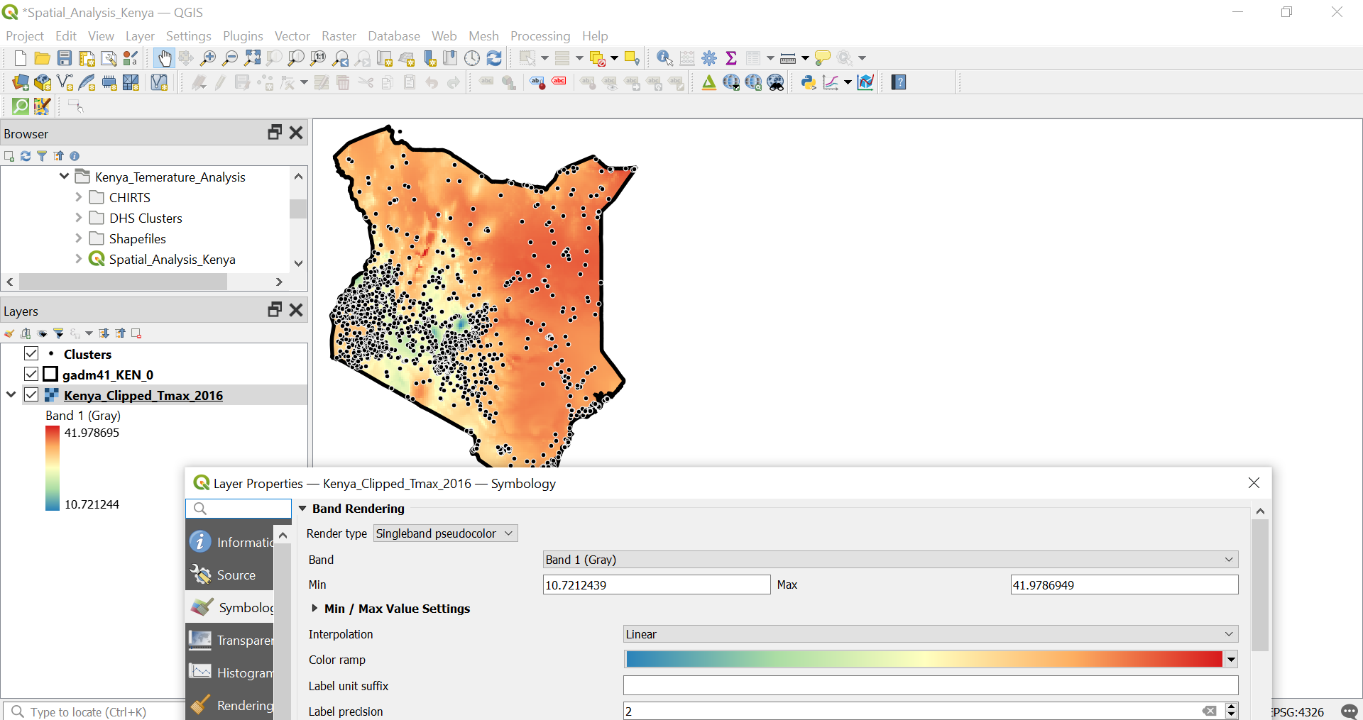
This map perfectly illustrates the synergy between the two data types. The raster provides the continuous environmental context (temperature), while the vector points provide the discrete locations of interest (clusters). This is a classic approach in spatial epidemiology, and one you will become very familiar with.

Conclusion

In this introductory lesson, we have established the fundamental concepts of spatial data. Let's summarize the key takeaways:

• Spatial data tells us where features are located.
• Vector data uses points, lines, and polygons to represent discrete objects with clear boundaries, like hospitals, roads, and administrative districts. Each vector feature has associated information stored in an attribute table.
• Raster data uses a grid of pixels to represent continuous surfaces without sharp boundaries, such as temperature, air pollution, or population density.

Understanding this distinction is the bedrock upon which all your future skills in spatial analysis will be built.

In our next lesson, we will address a logical follow-up question: Now that we know what these data types are, how does a computer know where to place them on the surface of the Earth? We will answer this by exploring the critical role of Coordinate Reference Systems (CRS) and map projections.