Understanding CRS and Map Projections in Health Mapping

The Fundamental Problem: From a Round Earth to a Flat Map

The core challenge of cartography and GIS is straightforward: the Earth is a three-dimensional sphere (more accurately, a slightly squashed and lumpy spheroid), while the maps we use—on paper or on a computer screen—are two-dimensional and flat. You cannot flatten the surface of a sphere without stretching, tearing, or squashing it. This unavoidable transformation process is called projection, and the result is always a compromise. Every flat map of the world distorts reality in some way.

To grasp this intuitively, watch the first part of the following video. It clearly defines what a map projection is and why distortion is an inevitable part of the process.

Step 1: Defining Location on a Sphere (Geographic Coordinate Systems)

Before we can make a flat map, we first need a reliable system for defining the location of any point on the Earth's 3D surface. This is the job of a Geographic Coordinate System (GCS). You are already familiar with its most common form: latitude and longitude.

A GCS uses a three-dimensional spherical model and measures locations in angular units (degrees). It's built from a few key components:

• Geoid: The true, highly complex, and irregular shape of the Earth, influenced by gravity. It's too bumpy to be used as a simple reference.
• Ellipsoid (or Spheroid): A simplified, mathematically defined smooth ellipse that approximates the geoid. Think of it as a perfect, smooth model of the Earth. The WGS 84 ellipsoid is the most famous example, used by all GPS systems.
• Datum: A datum defines the position of the ellipsoid relative to the geoid. It essentially "anchors" the smooth mathematical model to the real Earth, providing a frame of reference. Datums can be global (like WGS 84, which tries to be a best fit for the entire planet) or local (like NAD83, designed to be highly accurate for North America).

Data with different datums will not align correctly, even if they use the same ellipsoid! The following video provides an excellent visual breakdown of these concepts.

A GCS is perfect for storing spatial data and knowing its absolute position on the globe. However, because its units are degrees of an angle, it's not suitable for accurately measuring distances or areas in linear units like meters or kilometers. For that, we need to flatten the map.

Step 2: Flattening the Globe (Projected Coordinate Systems)

Once we have our data located on a 3D GCS, we can create a flat map using a Projected Coordinate System (PCS). A PCS is defined by:

1. A base GCS (like WGS 84 or NAD83).
2. A mathematical map projection method.

The projection transforms the angular latitude and longitude coordinates from the GCS into linear (x, y) coordinates on a flat Cartesian plane. These x, y coordinates are typically measured in meters or feet. This is what allows you to perform measurements on your map, such as calculating the area of a census tract or the distance between a patient's home and a hospital.

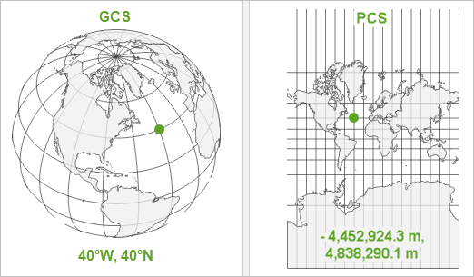
The image below perfectly illustrates this two-step reality. All spatial data starts with a GCS location on the globe, which is then projected into a PCS to be displayed on a flat map with a measurable grid.

The video you watched earlier also explains the different geometric shapes used for projection (cylinders, cones, and planes). These different methods produce different kinds of maps and, crucially, different kinds of distortions.

The Inevitable Trade-offs: Shape, Area, Distance, and Direction

Since all projections distort reality, a cartographer must choose what property to preserve at the expense of others. A projection can accurately preserve one or two of these properties, but never all of them for the whole map.

• Conformal (Preserves Shape): Local angles and shapes are preserved. This is vital for navigation. The famous Mercator projection is conformal. Its major drawback is that it massively distorts area, especially near the poles.
• Equal-Area (Preserves Area): The size of features on the map is proportional to their size on Earth. This is essential for most thematic health maps, where you might compare disease rates or population density across different administrative areas. To preserve area, these projections must distort shape. The Albers Equal Area Conic is a common choice for this.
• Equidistant (Preserves Distance): Preserves true scale and distance from one or two points to all other points on the map. Useful for creating buffers or service area rings around a specific point, like a clinic.
• Compromise: These projections don't preserve any single property perfectly but offer a good balance that minimizes overall distortion, making them suitable for general-purpose world maps. The Robinson projection is a popular example.

This article provides a concise explanation of these different projection types.

Why This Is Critical for Health Analysis

At this point, you might be thinking this is a niche technical detail. It is not. The choice of map projection can fundamentally change the results and interpretation of a spatial health analysis.

Let's watch a powerful demonstration. The Web Mercator projection, used by Google Maps, is conformal (preserves shape) but horribly distorts area. Watch how this affects a simple task like drawing a 500km circle on a map.

This visual proof is striking. A 500km buffer around a clinic in Canada would look vastly larger on a Mercator map than one in Mexico, even though they are the same size in reality. If you were to use such a map to visually estimate service coverage, your perception would be completely wrong.

Even more alarmingly, the choice of projection can alter the results of statistical tests. An academic paper explored this by applying different projections to the same health data.

The implications of this paper are profound. Your choice of projection could determine:

• Whether you find a statistically significant disease cluster or not.
• Where you believe a disease hotspot is located and how large it is.
• Your calculation of population density, which is the denominator for almost all disease rates.

This is the reason understanding projections is not optional for a spatial epidemiologist; it is a core methodological competency.

Conclusion

Let's recap the essential points from today's lesson.

• To locate data on Earth, we first use a Geographic Coordinate System (GCS), which uses latitude and longitude on a 3D model (an ellipsoid anchored by a datum).
• To create a flat, measurable map, we use a Projected Coordinate System (PCS), which mathematically transforms the GCS data onto a 2D surface.
• This projection process is a compromise and always introduces distortion in shape, area, distance, or direction.
• For health mapping, the choice of projection is a critical analytical decision. Using an equal-area projection is vital for thematic maps comparing rates or densities. Using the wrong projection can lead to incorrect measurements and, most alarmingly, can change the conclusions of statistical analyses like cluster detection.

You now understand the "what" (vector/raster) and the "where" (CRS/projections) of spatial data. In our next lesson, we will turn to a practical question: where do we find the data needed for health mapping? We'll explore common sources of spatial health data, such as census boundaries, health facility locations, and demographic information.