Data Integration for Unified Analysis

Introduction

In our last session, you learned how to clean individual datasets by identifying and handling missing values—a crucial first step for ensuring data quality. Now that you're equipped to prepare a single dataset, we'll address a very common real-world scenario: your data isn't in one place. Customer information might be in one file, their orders in another, and product details in a third.

This lesson focuses on a fundamental data preparation task: merging multiple datasets to create a unified view for analysis. You'll learn how to combine data from different sources into a single, cohesive pandas DataFrame. This skill is the bridge between collecting separate pieces of information and building a complete picture for analysis, which is essential for almost any data science project.

The Tools for Combining Data

Pandas provides three main functions for combining DataFrames: merge(), concat(), and join(). Each serves a different purpose.

This image provides a high-level overview of the three primary functions for combining DataFrames in pandas, highlighting their main use cases.

pd.merge(): This is the most flexible and powerful function, designed for database-style joining operations based on common columns (or "keys") or indices. We will focus most of our attention here.
pd.concat(): This function is best for stacking DataFrames on top of one another (vertically) or side-by-side (horizontally). It's like gluing datasets together along an axis.
DataFrame.join(): This is a convenience method for performing merges based on the DataFrame's index rather than columns. It's essentially a simplified version of pd.merge() for a common use case.

While all three are useful, mastering pd.merge() will cover the vast majority of your data combination needs.

Understanding Join Logic

The core concept behind merging is the "join". A join combines rows from two DataFrames based on a shared "key" column. The type of join you perform determines which rows are kept in the final result. There are four main types of joins.

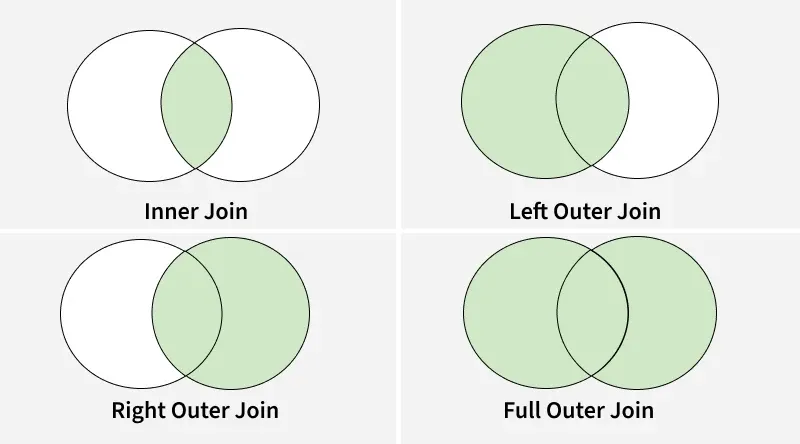
These Venn diagrams illustrate the logic of the four main join types. The shaded areas represent the data that is kept in the final merged DataFrame.

Let's break them down:

Inner Join (Default): Keeps only the rows where the key exists in both DataFrames. This is like finding the intersection of two sets. You'll lose any data that doesn't have a match.
Outer Join: Keeps all rows from both DataFrames. If a row from one DataFrame doesn't have a matching key in the other, the missing columns are filled with NaN (Not a Number). This is the union of two sets.
Left Join: Keeps all rows from the left DataFrame, plus any matching rows from the right DataFrame. If a row in the left DataFrame has no match in the right, the columns from the right DataFrame are filled with NaN.
Right Join: The opposite of a left join. It keeps all rows from the right DataFrame and fills in NaN for non-matching rows from the left.

To see a clear, simple demonstration of these four types in action, the following video is an excellent resource.

How do I merge DataFrames in pandas?

The presenter from Data School uses two very simple DataFrames to explain the logic of each join type, making the concepts easy to grasp.

Watch the segment on the four join types. As you watch, notice how the how parameter ('inner', 'outer', 'left', 'right') changes the final output and which rows are included or excluded.

The `pd.merge()` Function in Practice

Now that you understand the logic, let's dive into the practical implementation with pd.merge(). This function has a rich set of parameters that give you precise control over the merge operation. The best way to learn these is by seeing them applied.

The Python Data Science Handbook provides an excellent, concise guide to the key features of pd.merge().

Combining Datasets: Merge and Join

This chapter from Jake VanderPlas's handbook is a go-to reference for data professionals. It systematically walks through the functionality of pd.merge().

Please read the following sections: Categories of Joins: Start by reading the introduction to pd.merge() and then focus on the three subsections: Categories of Joins. This will show you how merges behave depending on the structure of your data (one-to-one, many-to-one, many-to-many). Specification of the Merge Key: Read this entire section, starting from Specification of the Merge Key. Pay close attention to the on, left_on, right_on, left_index, and right_index parameters. These are critical for telling pandas exactly how to match your DataFrames. Specifying Set Arithmetic for Joins: Read this section, which covers the how keyword. This directly implements the inner, outer, left, and right joins you saw in the video. Overlapping Column Names: Finally, read this short section on the suffixes keyword. This is a practical tool for handling a common issue where your DataFrames have identically named columns that are not the merge key.

A Real-World Workflow: Merging US States Data

Theory is one thing, but applying it to messy, real-world data is what matters. In your work, you'll frequently need to combine multiple files, clean up inconsistencies that arise from the merge, and then perform an analysis.

The following example from the same article demonstrates this entire workflow perfectly. It aims to rank US states by population density, but the necessary data (population, area, and state abbreviations) is spread across three separate files.

Combining Datasets: Merge and Join

This example is a mini-project that mirrors the exact process you'd follow in a professional setting. It combines merging with the data cleaning skills you learned in the previous lesson.

Please read the entire section, from the beginning to the end. As you follow along, pay special attention to these key steps in the workflow: First Merge (pop and abbrevs): Notice the use of how='outer', left_on, and right_on. Post-Merge Cleaning: The author immediately checks for nulls using .isnull().any() to find mismatches. This is a crucial validation step. The mismatched data (PR, USA) is then programmatically fixed. Second Merge (merged and areas): A second, simpler merge is performed using on='state'. Final Cleanup: The author again checks for nulls and decides to drop the remaining rows with missing data using dropna(). Analysis: Only after all the merging and cleaning is the final DataFrame used to calculate population density. This shows why merging is a data preparation step.

This end-to-end example is an excellent template for how to approach problems that require integrating data from multiple sources.

Clarifying `join()` and `concat()`

While pd.merge() is your most versatile tool, it's good to know when its cousins, join() and concat(), are more appropriate. join() is for convenient index-to-index merging, and concat() is for simple stacking.

Combining Data in pandas With merge(), .join(), and concat()

This article from Real Python provides a clear, high-level distinction between the three functions.

To round out your understanding, please read the introductory parts of these two sections: First, read the section on .join() to see how it simplifies index-based merges. Next, read the section on concat() to understand its role in stacking data.

This will help you recognize situations where these simpler functions are a more direct solution than a full pd.merge() call.

Conclusion

In this lesson, you've added a powerful set of tools to your data preparation arsenal. Combining disparate datasets is a foundational skill, and you are now equipped to handle it effectively.

Here are the key takeaways:

pd.merge() is your primary tool: It is highly flexible and can handle nearly any data-linking scenario you'll encounter.
The how parameter is crucial: The choice between 'inner', 'outer', 'left', and 'right' joins dictates how your data is combined and which rows are preserved.
Keys are everything: You must clearly specify how to match your DataFrames, using on for shared column names, left_on/right_on for different names, or left_index/right_index for index-based joins.
Merging is part of a workflow: A merge is often followed by a data validation step (like checking for nulls) to find and fix inconsistencies introduced by combining different sources.

In our next lesson, we will build directly on the unified DataFrame we've created. You will learn how to group and aggregate data to compute initial summary statistics. This will allow you to start summarizing your combined data to uncover high-level insights.

Recommended resources