Data Cleaning Techniques

1. Handling Missing Values: A Deeper Dive

In the last lesson, we saw how df.isnull().sum() can quickly reveal missing data (NaN values). Many machine learning algorithms cannot function with missing data, so we must address it. We briefly touched on dropna() and fillna(), but now let's explore these and other methods with more nuance.

Strategy 1: Deletion (dropna)

The most straightforward approach is to simply remove rows or columns containing NaN values. However, this can be a double-edged sword: while it's simple, you risk losing a significant amount of valuable data. Therefore, we should use it surgically.

The video below demonstrates how to use dropna more effectively by setting conditions.

• When to use dropna: Deletion is most appropriate when a row or column is missing a very large percentage of its data, or when the missing value is in a column so critical that the entire record is unusable without it. Using thresh gives you a great way to enforce a rule like "keep rows that have at least 5 valid data points."

Strategy 2: Imputation (Filling Values)

A more common and generally preferred strategy is imputation, which means filling in missing values with a calculated substitute. The goal is to make a reasonable guess that preserves the overall structure of the data.

Let's explore several imputation techniques, from simple to more sophisticated.

Let's summarize these imputation methods:

• Filling with a constant (fillna(0)): Simple, but can distort the column's statistics (like mean and standard deviation). Best used when 0 is a meaningful value (e.g., "0 items sold").
• Filling with a statistic (fillna(df['col'].mean())): A common choice for numerical data is to use the column's mean, median, or mode. The median is often preferred because it's less sensitive to outliers than the mean. The mode is the standard choice for categorical (non-numeric) data.
• Forward/Backward Fill (fillna(method='ffill')): This propagates the last known value forward (ffill) or the next known value backward (bfill). This is especially useful in time-ordered data where you can assume a value remained constant until the next measurement.
• Interpolation (interpolate()): This is often the most sophisticated approach for numerical data. It treats the missing point as being on a line between its neighbors. As you saw, method='linear' estimates a value evenly between its neighbors, while method='time' accounts for the actual time gap, providing a more accurate estimate for time-series data.

Choosing the right method depends on the nature of your data and the reason it's missing.

2. Handling Duplicates (Review and Extend)

We covered df.drop_duplicates() in the last lesson. Let's quickly review and add a crucial detail. Duplicates can arise from data entry errors or system glitches, and they can bias your analysis by giving extra weight to the duplicated records.

A common real-world scenario is when a row is not a complete duplicate, but is a duplicate based on a key identifier. For example, you might have two records for the same customer ID but with different timestamps. You may want to keep only the most recent one. You can handle this by specifying which columns to consider when checking for duplicates.

# Create a sample DataFrame
data = {'user_id': [101, 102, 101, 103],
        'action': ['login', 'browse', 'login', 'logout']}
df = pd.DataFrame(data)




# Show duplicates based on all columns (there are none)
print("Complete duplicates:", df.duplicated().sum())




# Show duplicates based only on 'user_id'
print("Duplicates by user_id:", df.duplicated(subset=['user_id']).sum())




# Drop duplicates based on 'user_id', keeping the first instance
df_unique_users = df.drop_duplicates(subset=['user_id'], keep='first')
print(df_unique_users)

The subset parameter is extremely useful for ensuring data integrity based on your dataset's unique identifiers.

3. Handling Outliers

Now we turn to a new and important topic: outliers. An outlier is a data point that deviates significantly from the rest of the observations. They can be caused by measurement errors, data entry mistakes, or genuinely rare events.

Why do we care? Outliers can:

• Distort statistical measures like the mean and standard deviation.
• Disproportionately influence the training of machine learning models, leading to poor performance (especially for linear models and anything distance-based).

Detecting and Handling Outliers

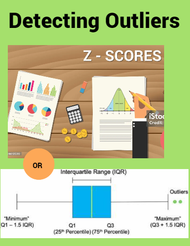
We can use statistical rules to flag data points as outliers. Two of the most common methods are the Z-score and the Interquartile Range (IQR).

The following video provides an excellent, practical walkthrough of how to implement these methods in Python. It also introduces the key decision you must make when you find an outlier: trimming (removing it) or capping (replacing it with a less extreme value).

Let's recap the key ideas:

• Z-Score: Measures how many standard deviations a data point is from the mean. A common rule of thumb is to consider anything with a Z-score greater than 3 or less than -3 as an outlier. This method works best when your data is approximately normally distributed (a bell curve).
• IQR Method: This method defines outliers based on the interquartile range (IQR = Q3 - Q1). Any point below Q1 - 1.5 * IQR or above Q3 + 1.5 * IQR is flagged. Because it uses the median and quartiles, it is not affected by the presence of extreme outliers, making it a more robust choice for skewed data.
• Trimming vs. Capping:
  • Trimming: Deleting the outlier row. This is simple but results in data loss.
  • Capping (or Winsorization): Replacing outlier values with the nearest "acceptable" value (i.e., the upper or lower boundary you calculated). This is often preferred as it retains the record while reducing the influence of the extreme value.

The choice of method and whether to trim or cap depends on your specific goals and domain knowledge. If an outlier is due to a clear error, removing it might be best. If it's a genuine but rare event, capping might be more appropriate.

Conclusion

Excellent work! You've now moved beyond basic cleaning and have a robust set of tools for handling some of the most common and challenging data quality issues.

Key Takeaways:

• For missing values, you can choose between controlled deletion (dropna with thresh) or various imputation methods like fillna (with mean/median/mode), forward/backward fill (ffill/bfill), or interpolate() for more accurate estimates.
• Duplicates can be removed based on all columns or, more practically, on a subset of key identifier columns.
• Outliers are extreme values that can harm your analysis. You can systematically detect them using statistical methods like Z-score and IQR.
• When an outlier is found, you have a choice: trim (remove) it or cap (replace) it to mitigate its effect without losing the entire record.

In our next lesson, we will address another common data preparation task: combining data. Real-world projects rarely rely on a single data file. You'll learn how to use pandas to merge, join, and concatenate multiple DataFrames to build a comprehensive dataset for analysis.