Transfer Learning with ResNet and VGG

1. What is Transfer Learning?

Imagine you're training a model to classify different types of flowers. To do this from scratch, your model would first need to learn to recognize basic visual features like edges, corners, colors, and textures. Then, it would learn to combine these into more complex features like petals, stems, and leaves, before finally learning to distinguish between a rose and a tulip. This process can take millions of images and weeks of training.

Transfer learning offers a powerful shortcut. We can take a model that has already been trained on a very large and diverse dataset (like ImageNet, which has over a million images and 1000 categories), and adapt it for our own task. This pre-trained model has already learned a rich hierarchy of visual features. We are essentially transferring its "knowledge" of the visual world to our specific problem.

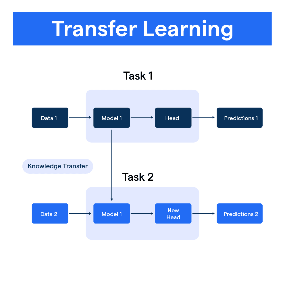
Let's start with a short reading that introduces this concept more formally.

There are two primary ways to apply transfer learning:

1. ConvNet as a Fixed Feature Extractor: We take the pre-trained model and "freeze" all of its layers. We then remove the original final classification layer and add a new one that is customized for our task (e.g., classifying ants vs. bees instead of 1000 ImageNet classes). During training, only the weights of this new layer are updated. The pre-trained network acts as a sophisticated, fixed feature extractor.
2. Fine-Tuning: This approach goes a step further. We not only replace and train the final layer but also "unfreeze" some of the later layers of the pre-trained model. We then continue training these layers on our new data, but with a very low learning rate. This allows the model to subtly adjust its pre-learned features to better suit the specifics of our new dataset.

The official PyTorch tutorial explains these two scenarios concisely.

In this lesson, we will focus on the first method: using the ConvNet as a fixed feature extractor. We will cover fine-tuning in detail in our next lesson.

2. Transfer Learning as a Feature Extractor: The Workflow

Let's break down the practical steps for implementing the feature extraction method in PyTorch.

1. Load a Pre-trained Model: PyTorch's torchvision.models library gives us easy access to many famous, pre-trained models like ResNet, VGG, DenseNet, and more. We can load one with a single line of code, specifying that we want the weights pre-trained on ImageNet.

2. Freeze the Model's Layers: To use the model as a fixed feature extractor, we must prevent its weights from being updated during training. We do this by iterating through all the model's parameters and setting their requires_grad attribute to False.

3. Replace the Classifier: The pre-trained model has a final fully-connected layer (the "classifier" or "head") designed for its original 1000 classes. We must replace this with a new nn.Linear layer whose output dimension matches the number of classes in our dataset. By default, new layers have requires_grad=True, so only this new layer will be trained.

4. Train: We set up our optimizer to only work on the parameters of the new classifier head and run the training loop. The forward pass goes through the entire network, but the backward pass and weight updates only apply to our new layer.

This video provides a complete, practical walkthrough of this entire process.

3. Code Implementation in PyTorch

To solidify your understanding, let's examine the code from the official PyTorch tutorial, which implements the same feature extraction strategy. This approach is slightly more explicit in how it configures the optimizer, which is a common and efficient practice.

Here is a summary of the key code snippet you just reviewed, which represents the core logic of transfer learning via feature extraction:

# 1. Load a pre-trained model
model_conv = torchvision.models.resnet18(weights='IMAGENET1K_V1')




# 2. Freeze all the parameters in the network
for param in model_conv.parameters():
    param.requires_grad = False




# 3. Replace the final layer for our new task
# Get the number of input features for the classifier
num_ftrs = model_conv.fc.in_features



# Create a new layer with the correct number of output classes
model_conv.fc = nn.Linear(num_ftrs, len(class_names)) 




# Move the model to the device (CPU or GPU)
model_conv = model_conv.to(device)




# 4. Set up the optimizer to only train the new classifier
# Note: only parameters of the final layer are being optimized
optimizer_conv = optim.SGD(model_conv.fc.parameters(), lr=0.001, momentum=0.9)




# ... then proceed with your standard training loop

This pattern is incredibly powerful and is a standard first step when tackling almost any image classification problem. It's efficient, effective, and allows you to build high-quality models quickly.

Conclusion

Congratulations! You've just learned one of the most impactful techniques in modern AI. By leveraging the knowledge stored in massive, pre-trained models, you can bypass the immense cost of training from scratch and build highly accurate computer vision systems with a fraction of the data and effort.

Key Takeaways:

• Transfer learning is the process of adapting a model trained on one task for a second, related task.
• It is a standard practice in computer vision because it saves enormous amounts of training time and data, while leading to better results.
• The feature extraction method involves freezing the weights of a pre-trained model and training only a new, custom-built classification head.
• The key steps in PyTorch are:
  1. Load a model from torchvision.models with pre-trained weights.
  2. Set param.requires_grad = False for all parameters you want to freeze.
  3. Replace the final classification layer (model.fc in ResNet) with a new one matching your number of classes.
  4. Configure the optimizer to only update the parameters of your new layer.

Preview of the Next Lesson:
The feature extraction method is a fantastic starting point. However, we can often squeeze out even more performance by allowing the model to adapt its learned features more closely to our new data. In the next lesson, "Fine-tune pre-trained models on custom datasets," we will explore how to unfreeze some of the pre-trained layers and train them gently to achieve state-of-the-art results.