Estimating Biexciton Binding Energies Using Variational Methods

1. The Variational Principle: A Refresher

Given your background in multiple quantum mechanics courses, you're certainly familiar with the variational principle. It's one of the most powerful tools in quantum physics for estimating the ground state energy of a system when the Schrödinger equation is too complex to solve exactly.

The core theorem states that for any normalized trial wavefunction ${\Psi }_T$, the expectation value of the Hamiltonian provides an upper bound to the true ground state energy $E_0$:
$E[{\Psi }_T]=⟨{\Psi }_T|H|{\Psi }_T⟩\ge E_0$
The method, then, is to choose a "guess" wavefunction ${\Psi }_T$ with some adjustable parameters $\{{\alpha }_1,{\alpha }_2,...\}$, calculate the energy functional $E(\{{\alpha }_i\})$, and then minimize this energy with respect to the parameters. The better our guess, the closer the resulting minimum energy will be to the true ground state energy.

For a quick and effective review of the principle and its proof, please watch the following video.

2. Crafting a Biexciton Trial Wavefunction

The success of the variational method hinges entirely on the quality of the trial wavefunction. A good ${\Psi }_T$ must capture the essential physics of the system. For a biexciton, this means it must account for:

1. The two internal exciton structures.
2. The repulsive interactions between like charges (e1-e2, h1-h2).
3. The overall exchange symmetry requirements (antisymmetric for electron exchange and for hole exchange).
4. The correlation between all four particles.

As we discussed last time, the biexciton ground state is typically a spin-singlet for both electrons and holes. This means the spin part of the wavefunction is antisymmetric, so the spatial part must be symmetric under the exchange of electron coordinates (${\mathbf{r}}_{e1}\leftrightarrow {\mathbf{r}}_{e2}$) and hole coordinates (${\mathbf{r}}_{h1}\leftrightarrow {\mathbf{r}}_{h2}$).

A classic and highly effective form for the biexciton wavefunction was proposed by Hylleraas and Ore, and modern variations build upon it. Let's examine a sophisticated trial wavefunction used in recent research on perovskite nanoplatelets. This will give you a concrete sense of how these functions are constructed in practice.

Let's break down the structure of the wavefunction ${\Psi }_{BX}$ from the paper:

${\Psi }_{BX}=N_{BX}{\Phi }_e({\mathbf{r}}_1,{\mathbf{r}}_2){\Phi }_h({\mathbf{r}}_a,{\mathbf{r}}_b)F({\mathbf{r}}_1,{\mathbf{r}}_2,{\mathbf{r}}_a,{\mathbf{r}}_b)$

• ${\Phi }_e$ and ${\Phi }_h$ are the non-interacting electron and hole envelope functions, which primarily account for the quantum confinement within the nanostructure.
• $F$ is the crucial correlation factor, which contains the variational parameters and describes the inter-particle dynamics.

The correlation factor $F$ has the form:
$F\sim e^{-Z(s_1+s_2)/2}\cosh (Q(t_1-t_2)/2)\times (\text{repulsion terms})$

• The first term, $e^{-Z(s_1+s_2)/2}$, is reminiscent of the hydrogenic ground state wavefunction. Here, $s_1=r_{1a}+r_{1b}$ and $s_2=r_{2a}+r_{2b}$ represent the sum of distances of each electron to both holes. The parameter $Z$ acts as an effective charge, scaling the strength of the electron-hole attraction and controlling the overall size of the complex.
• The $\cosh$ term contains the parameter $Q$. This term is fascinating:
  • If $Q=0$, the wavefunction is symmetric and describes a tightly bound, square-like molecule.
  • If $Q=1$, the wavefunction separates into two independent excitons.
  • Thus, $Q$ is a variational parameter that allows the system to find the optimal balance between a single molecular entity and two weakly interacting excitons.
• The final terms, which the paper calls Padé-Jastrow factors, explicitly model the repulsion between like charges (e-e and h-h) using parameters $\alpha$ and $\beta$.

This structure provides a flexible and physically intuitive framework for approximating the true ground state.

3. Calculating the Energy: The Role of Computation

With the Hamiltonian $H_{XX}$ from the previous lesson and the trial wavefunction ${\Psi }_T$, the next step is to compute the energy functional:
$E(Z,Q,\alpha ,\beta )=\frac{\int {\Psi }_T^{\ast }{H}_{XX}{\Psi }_T{d}^{12}\mathbf{r}}{\int |{\Psi }_T{|}^2{d}^{12}\mathbf{r}}$
This is a 12-dimensional integral, which is impossible to solve analytically. This is where your computational physics background becomes highly relevant. Such integrals are almost always evaluated using numerical methods, with Variational Monte Carlo (VMC) being a standard choice.

The paper you just read on perovskites explicitly states this:

"A straight variational solution of ΨBX is not viable because of the large number of dimensions. We then resort to a Quantum Monte Carlo integration..."

The VMC method uses a random walk to sample points in the 12D configuration space according to the probability distribution $|{\Psi }_T{|}^2$, allowing for an efficient estimation of the integral. The parameters $(Z,Q,\alpha ,\beta )$ are then optimized numerically to find the minimum energy.

An Alternative: The Linear Variational Method

Another powerful computational approach is the linear variational method. Instead of a single complex function, the trial wavefunction is expressed as a linear combination of simpler basis functions ${\varphi }_i$:
${\Psi }_T={\sum }_{i=1}^N{c}_i{\varphi }_i$
Here, the coefficients $c_i$ are the variational parameters. Applying the variational principle to this form transforms the problem of solving a differential equation into a problem of linear algebra: finding the eigenvalues of a matrix.

This method leads to the generalized eigenvalue problem:
$\mathbf{Hc}=E\mathbf{Sc}$
where $\mathbf{H}$ is the Hamiltonian matrix with elements $H_{ij}=⟨{\varphi }_i|H|{\varphi }_j⟩$, $\mathbf{S}$ is the overlap matrix with elements $S_{ij}=⟨{\varphi }_i|{\varphi }_j⟩$, and $\mathbf{c}$ is the vector of coefficients. Solving for the lowest eigenvalue $E$ gives the best estimate of the ground state energy for the chosen basis set.

The following video provides a clear derivation of this matrix equation.

4. From Energy to Binding Energy: Case Studies

Once the minimization procedure yields the estimated biexciton ground state energy, $E_{XX}$, we can finally calculate the quantity of physical interest: the biexciton binding energy, $E_B$.

$E_B=2E_X-E_{XX}$

A positive $E_B$ indicates a stable biexciton. Spectroscopically, this binding energy appears as the energy difference between the exciton emission peak and the biexciton emission peak, as the biexciton decays into an exciton and a photon.

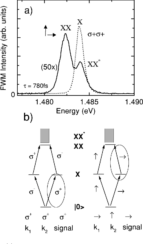
Let's see how the variational calculations stack up against experimental reality in the materials you're interested in.

Case 1: Biexcitons in Perovskite Nanoplatelets

The perovskite paper provides a perfect example. After performing the VMC calculation, they find the binding energy and analyze how it changes with the thickness of the nanoplatelet.

As the paper shows, the variational method successfully predicts that the biexciton binding energy increases dramatically as the system becomes more 2D (thinner nanoplatelets). This is a direct consequence of quantum confinement enhancing the Coulomb interactions. This trend is a general feature in nanostructures.

Case 2: Biexcitons in Cuprous Oxide (Cu₂O)

The variational method is also crucial for understanding biexcitons in bulk materials like Cu₂O, which is a key system for your research interests.

The following paper on quadrupole biexcitons in Cu₂O explicitly uses the variational principle to find the biexciton energies.

This demonstrates the wide applicability of the variational method, from quasi-2D perovskites to bulk Cu₂O, providing theoretical estimates that can be directly compared with spectroscopic measurements.

Conclusion

In this lesson, we have bridged the gap between formulating the biexciton Hamiltonian and calculating its physical properties. The variational principle provides a robust and computationally feasible path to estimating the ground state energy of this complex four-body system.

Key Takeaways:

• The variational principle allows us to find an upper bound for the biexciton ground state energy by minimizing the energy expectation value of a parameterized trial wavefunction.
• A good trial wavefunction must be physically motivated, respecting symmetries (like spin exchange) and including parameters that capture key physics like electron-hole attraction ($Z$), inter-exciton coupling ($Q$), and like-charge repulsion ($\alpha ,\beta$).
• The high-dimensional integrals involved necessitate numerical methods, such as Variational Monte Carlo or solving the generalized eigenvalue problem that arises from the linear variational method.
• By calculating the minimized biexciton energy $E_{XX}$, we can find the biexciton binding energy $E_B=2E_X-E_{XX}$, a key quantity measured in optical spectroscopy.

Preview of the Next Lesson

We have now established how to find the energy and wavefunction of a biexciton. The next logical step is to understand how we create and observe these states in the lab. In the next lesson, we will focus on the learning outcome: "Derive the selection rules for biexciton creation via two-photon absorption and decay via radiative cascade." We will explore the quantum mechanical rules that govern how light interacts with biexcitons, connecting our theoretical model directly to experimental observables.