Quick Sort: Pivoting and Performance

1. The Core Idea: Pick a Pivot and Partition

Like Merge Sort, Quick Sort uses the divide-and-conquer approach. However, it shifts the main "work" to the "divide" step, not the "combine" step. The process is as follows:

1. Pick a Pivot: Choose one element from the array. This element is called the pivot. The strategy for choosing the pivot is crucial, and we'll discuss it in detail.
2. Partition: Rearrange the array so that all elements smaller than the pivot are to its left, and all elements greater than the pivot are to its right. After this step, the pivot element is in its final, correct sorted position.
3. Recurse: Recursively apply the Quick Sort algorithm to the two sub-arrays: the one to the left of the pivot and the one to the right.

The key insight is that once the pivot is in its correct place, it never needs to be moved again. The problem is now reduced to sorting the two smaller, independent sub-arrays.

Let's watch Striver's explanation. He masterfully breaks down this core intuition.

2. The Partition Function: The Heart of Quick Sort

The most intricate part of Quick Sort is the partition function. Its job is to take an array (or sub-array) and a chosen pivot, and perform the rearrangement we just described. A common and efficient way to do this in-place is by using two pointers.

Striver's preferred method, which aligns with your course structure, involves:

1. Choosing the first element (arr[low]) as the pivot.
2. Initializing two pointers, i at low and j at high.
3. Moving i forward until you find an element > pivot.
4. Moving j backward until you find an element <= pivot.
5. If i is still to the left of j, swap arr[i] and arr[j].
6. Repeat until the pointers i and j cross.
7. Once they cross, swap the pivot (arr[low]) with arr[j]. The pivot is now at its correct sorted position, and the function returns this index (j).

Let's see the pseudocode and a dry run of this partitioning logic. This will clarify how the array is rearranged without using extra memory.

3. Implementation in Java

With the partition logic clear, we can assemble the full Quick Sort algorithm. It consists of two main parts:

• quickSort(arr, low, high): The recursive function that checks the base case (low >= high) and orchestrates the process. It calls partition to get the pivot's final index and then recursively calls itself for the left and right sub-arrays.
• partition(arr, low, high): The function we just studied, which rearranges the sub-array and returns the pivot's index.

The following resource from takeuforward.org provides a clean Java implementation that directly reflects the logic from Striver's video.

4. Performance: Average vs. Worst Case

Here is where Quick Sort reveals its complex personality. Unlike Merge Sort, its performance is not a constant guarantee.

Average-Case Performance: $O(n\log n)$

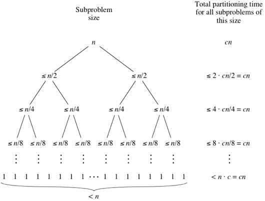
The ideal scenario for Quick Sort is when the pivot choice consistently divides the array into two roughly equal halves. If the pivot is always the median element, each partition creates two sub-problems of size n/2.

• Partitioning Work: The partition function scans the sub-array, which takes linear time, $O(n)$.
• Recursion Depth: Halving the problem at each step results in a recursion depth of $O(\log n)$.

This leads to the same recurrence relation as Merge Sort, $T(n)=2T(n/2)+O(n)$, which resolves to $O(n\log n)$. Even if the splits are not perfectly balanced (e.g., a 10%-90% split), the time complexity remains $O(n\log n)$. This efficient performance is what we observe on average with a good pivot strategy.

Worst-Case Performance: $O(n^2)$

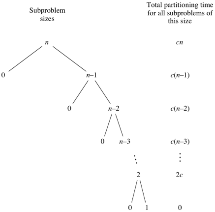
The worst-case scenario occurs when the chosen pivot is consistently the smallest or largest element in the sub-array. This leads to extremely unbalanced partitions. A common trigger for this is trying to sort an already sorted (or reverse-sorted) array while always picking the first or last element as the pivot.

In this case, the partition step splits the array of size k into two sub-arrays of sizes 0 and k-1.

• Partitioning Work: Still takes linear time, $O(k)$.
• Recursion Depth: The problem size only decreases by one at each step, leading to a recursion depth of $O(n)$.

The total work becomes a sum of an arithmetic series: $O(n)+O(n-1)+...+O(1)$, which is $O(n^2)$.

This performance disparity highlights the importance of the pivot selection strategy. While picking the first or last element is simple to code, it's vulnerable. A common and more robust technique is to pick a random pivot. This makes the worst-case scenario statistically very unlikely, as it's improbable to randomly pick the worst pivot every single time. Another popular method is the "median-of-three" strategy, where you take the first, middle, and last elements and choose their median as the pivot.

For a formal analysis, the Baeldung article provides a concise explanation.

Space Complexity

Quick Sort's main advantage over Merge Sort is its space efficiency.

• It operates in-place, so it doesn't require an $O(n)$ auxiliary array.
• The space it uses comes from the recursion call stack.
  • Average Case: The recursion depth is $O(\log n)$, so the space complexity is $O(\log n)$.
  • Worst Case: The recursion depth is $O(n)$, leading to a space complexity of $O(n)$.

This makes Quick Sort a preferred choice when memory is a concern, as its average-case space usage is excellent.

Conclusion

In this lesson, we've dissected Quick Sort, a powerful but variable sorting algorithm. It exemplifies a different flavor of divide-and-conquer where the intelligence lies in the partitioning step.

Key Takeaways:

• Core Logic: Quick Sort works by picking a pivot, partitioning the array around it, and then recursively sorting the two resulting sub-arrays.
• In-Place Sorting: Its primary advantage is sorting in-place, giving it an average space complexity of $O(\log n)$.
• Pivot is Key: The choice of pivot is critical. A good pivot leads to balanced partitions and $O(n\log n)$ time complexity.
• Worst-Case: A poor pivot strategy (e.g., on an already sorted array) can lead to highly unbalanced partitions and degrade performance to $O(n^2)$. Randomizing the pivot is a standard way to mitigate this risk.

We have now covered the most important "from-scratch" sorting algorithms. In our next lesson, we will shift our focus to practical application. You will learn how to use Java's built-in sorting methods, Arrays.sort() and Collections.sort(), and, importantly, how to customize their behavior for complex objects using custom Comparators. This is an essential skill for real-world programming and competitive coding.