In our last lesson, we established the conceptual foundation of epidemiology, distinguishing between prevalence (the burden of existing disease) and incidence (the risk of new disease). We used the "epidemiologist's bathtub" analogy to understand how these two measures relate to each other and to disease duration.
Now, we will move from concepts to calculations. Your goal for this lesson is to learn how to calculate and, just as importantly, correctly interpret the three fundamental measures of disease frequency: prevalence, cumulative incidence, and the incidence rate. Mastering these calculations is the first step toward the quantitative analysis that underpins all epidemiological studies.
A Quick Recap: The "Bathtub" Model
Let's briefly revisit the relationship between incidence and prevalence.
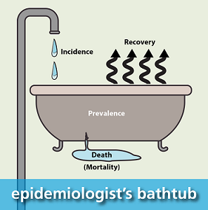
As this model shows, the total number of people with a disease at any time (prevalence) depends on how many new people get it (incidence) and how long they stay sick. Now, let's learn how to put numbers to these concepts.
Calculating Prevalence
As we discussed, prevalence is a snapshot of the proportion of a population that has a disease at a specific point in time. It's a simple proportion.
The formula is:
Let's review the calculation with a clear example.
Measures of Disease Frequency – Foundations of Epidemiology
This section of the "Foundations of Epidemiology" textbook provides worked examples for calculating prevalence.
Please read the section on Prevalence, starting from its definition up to the end of the second example, the breastfeeding example. Pay close attention to how the denominator is defined in each case.
The key to interpreting prevalence is to be specific about the population and the time point. For instance, a prevalence of 8% is interpreted as: "At that specific time, 8% of the student population living in the dorms had the flu." This measure is vital for healthcare planning and resource allocation.
Calculating Incidence: Two Essential Methods
Measuring incidence—the occurrence of new cases—is more complex because it involves time. The population must be followed over a period to see who develops the disease. There are two primary ways to calculate incidence, each suited to different study conditions.
- Cumulative Incidence (or Incidence Proportion): Used for "closed" populations where everyone is followed for the same amount of time.
- Incidence Rate: Used for "dynamic" populations where people are followed for different lengths of time.
1. Cumulative Incidence (Incidence Proportion)
Cumulative incidence measures the proportion of an at-risk group that develops a disease over a specified follow-up period. It's often simply called risk.
The formula is:
The denominator here is critical: it only includes individuals who are at risk of developing the disease at the beginning of the study. We exclude anyone who already has the disease or is immune.
Measures of Disease Frequency – Foundations of Epidemiology
The textbook we've been using offers a great introduction to cumulative incidence, which it calls "Incidence Proportion."
Read the section on Incidence, focusing on the part that defines and explains Incidence Proportion. Then, work through the first example about flu in a classroom. Notice how the prevalent case is removed from the denominator.
When you calculate a cumulative incidence of 8.3 per 100, the interpretation is: "The average risk of developing the flu for students in that class over that specific week was 8.3%." This measure gives a straightforward estimate of risk for a defined group over a defined period.
2. Incidence Rate (Incidence Density)
The cumulative incidence calculation assumes we can follow everyone for the entire study period. In reality, this is rare. People may enter a study at different times, move away, be lost to follow-up, or die from other causes. This creates a "dynamic" population with unequal follow-up times. Your background in data science has likely prepared you for the challenges of working with such incomplete or "messy" real-world data.
To handle this, we use the Incidence Rate. Instead of just counting people in the denominator, we sum up the total amount of time that each person was observed and remained at risk. This sum is called person-time.
The formula is:
Person-time is often measured in person-years, person-months, or person-days. The resulting rate is not a proportion and can range from 0 to infinity. It represents the "speed" at which new cases are occurring in the population.
Calculating person-time can seem tricky at first, but it's a systematic process of accounting. The following resources provide an excellent, step-by-step guide.
Measures of Disease Frequency – Foundations of Epidemiology
This part of the textbook walks through a detailed graphical example of how to calculate person-time and the resulting incidence rate.
Read the section beginning with the definition of incidence rate. Carefully follow the breakdown of how each of the 10 people in Figure 2-3 contributes to the total person-months at risk. Then, review the final calculation of the rate.
To reinforce this crucial concept, the following video provides a visual walkthrough of calculating incidence in a dynamic population.
Epidemiology: Measure of Disease Frequency, Incidence and Prevalence
This video from the UTAH Center for Clinical & Translational Science explains the concept of person-time using animated graphics, which can help solidify your understanding.
Watch the segment from the explanation of dynamic populations. Pay attention to how the varying follow-up times for each individual are summed to create the person-time denominator.
The key interpretation for an incidence rate is centered on the person-time unit. For example, a rate of "4.14 per 10 person-years" means that for every 10 years of 'at-risk' observation time accumulated by the population, we would expect to see about 4 new cases.
Tying It All Together: A Visual Example
The table below from the epidemiology textbook provides a concise summary comparing the two types of incidence measures.
Measures of Disease Frequency – Foundations of Epidemiology
This table is a useful quick reference for the key differences between incidence proportion (risk) and incidence rate.
Review Table 2-1 in its entirety.
Now, let's analyze a single diagram that calculates all three measures for the same hypothetical cohort. This will help you see how the choice of denominator changes the resulting measure and its interpretation.

Let's break down the calculations shown in the image:
-
Cumulative Incidence Proportion:
- Numerator: 2 individuals experience Event Y.
- Denominator: 8 individuals were at risk at the start of the study.
- Calculation: .
- Interpretation: The risk of experiencing Event Y over the one-year period was 25%.
-
Incidence Rate for Event Y:
- Numerator: 2 individuals experience Event Y.
- Denominator (Person-Time): Event Y happens at the very end of the study for both individuals. Therefore, all 8 people were followed for the full year. The total person-time is person-years.
- Calculation: cases per person-year.
- Interpretation: The rate of Event Y was 0.25 cases for every person-year of observation.
-
Incidence Rate for Event X:
- Numerator: 2 individuals experience Event X.
- Denominator (Person-Time): This is different! The two events occur at the 6-month mark (0.5 years). After the event, those individuals are no longer 'at risk' and their observation time stops contributing to the denominator.
- The total person-time is person-years. (Note: The image mistakenly omits the final person's full year of observation time in the denominator string, but the total '7' is correct based on the logic: 5 full years + 2 half years).
- Calculation: cases per person-year.
- Interpretation: The rate of Event X was approximately 0.29 cases for every person-year of observation.
This example powerfully illustrates how the incidence rate, by using person-time, provides a more precise measure of incidence when follow-up time is variable.
Conclusion
In this lesson, you've added the essential skill of calculation to your conceptual understanding of disease frequency. You can now quantify the burden and risk of disease in a population.
Here are the key takeaways:
- Prevalence is a proportion of existing cases at a point in time. It is calculated as
Cases / Total Population. - Cumulative Incidence (Risk) is a proportion of new cases over a period in a closed population. It is calculated as
New Cases / Population at Risk at Start. - Incidence Rate measures the speed of new cases in a dynamic population. It is calculated as
New Cases / Total Person-Time at Risk. The concept of person-time is crucial for accurately handling variable follow-up periods.
In our next lesson, we will put these measures to work. We will learn how to calculate measures of association, such as the Risk Ratio and Rate Ratio. These measures allow us to compare the frequency of disease between two or more groups, forming the analytical core of most epidemiological studies.