Welcome to the next lesson in our module on confounding. In our previous discussion, we focused on proactive strategies to control for confounding at the study design stage, such as randomization and matching. These methods are our best defense, but they aren't always possible. What do we do when we analyze data from a study where confounding might still be present?
This lesson transitions from study design to study analysis. We will tackle the learning outcome: Assess confounding by comparing crude and adjusted estimates of association. You will learn a fundamental analytical technique called stratification to determine whether a variable is distorting the relationship you're investigating. This process is conceptually similar to how in machine learning you might evaluate a simple model, then add a new variable and re-evaluate to see how it changes the model's parameters and overall interpretation.
Crude vs. Adjusted Estimates: Seeing Through the Noise
Before we dive into the method, let's clarify two key terms:
- A crude estimate of association (like a crude odds ratio or risk ratio) is the measure calculated using only the exposure and outcome variables. It's our initial, "unadjusted" look at the data, and it may be distorted by confounders.
- An adjusted estimate is a measure of association that has been statistically corrected to remove or "control for" the effect of one or more confounding variables. It provides a more accurate picture of the true relationship between the exposure and outcome.
Think of the crude estimate as a noisy signal. Our goal is to apply an analytical filter—in this case, stratification—to remove the noise (confounding) and reveal the cleaner, adjusted signal underneath.
The following short video introduces this idea of "adjustment" using the example of age-confounded death rates. It demonstrates how an overall (crude) rate can be misleading and how creating an adjusted rate reveals the true underlying risk.
The role of adjustment in age confounding
This video from Medmastery provides an excellent conceptual introduction to adjustment.
Watch the entire video. Pay attention to how the crude death rate in City A is misleading (the initial problem) and how applying the age-specific rates to a standard population creates an "age-adjusted" rate that allows for a fair comparison (the adjustment process).
The Stratification Method for Assessing Confounding
Stratified analysis is the method we use to move from a crude estimate to an adjusted one and, in the process, determine if confounding is present. The logic is to isolate the effect of a potential confounder by looking at the exposure-outcome relationship within different levels, or strata, of that variable.
The overall process can be visualized as follows:
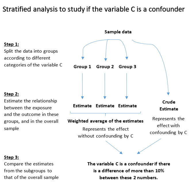
Let's walk through this process with a detailed example. We'll use an excellent chapter from the Foundations of Epidemiology textbook by Oregon State University.
Confounding – Foundations of Epidemiology
This resource provides a clear, step-by-step example of assessing confounding using stratification. We will follow its logic closely.
First, read the introductory part of the section on analytical control methods. Focus on the case-control study example introduced in "To stratify...". Here, the author calculates the crude odds ratio for the association between oral contraceptive (OCP) use and ovarian cancer. This is our starting point. Next, follow the author's logic as they check the criteria for smoking to be a potential confounder. The core of the analysis begins with stratification. Read carefully as the data is split into two tables: one for smokers and one for non-smokers. Finally, examine the calculation of the stratum-specific odds ratios. Pay close attention to the comparison: the two stratum-specific ORs (0.44) are similar to each other, but very different from the crude OR (1.0). This is the classic signature of confounding.
The Rule of Thumb: The 10% Change Criterion
As you saw in the reading, the key sign of confounding is a meaningful difference between the crude estimate and the adjusted estimate (which is derived from the similar stratum-specific estimates). But how much of a difference is "meaningful"?
In epidemiology, a common rule of thumb is the 10% change criterion. If the adjusted estimate is different from the crude estimate by 10% or more, we conclude that there is confounding.
The formula is:
In our OCP-cancer example:
- Crude OR = 1.0
- Adjusted OR (represented by the stratum-specific ORs) = 0.44
Plugging this into the formula:
Since 127% is much greater than 10%, we can confidently conclude that smoking is confounding the relationship between OCP use and ovarian cancer. The crude OR of 1.0 is biased, and the adjusted OR of 0.44 is the more accurate measure of the association.
A Framework for Decision-Making
The process of assessing confounding involves a series of comparisons. The flowchart below provides a comprehensive map for this decision-making process. For today, we are focusing on the path that leads to identifying confounding.
Let's watch a short video clip that reinforces this logic. While the video's main topic is effect modification (which we will cover later), it does an excellent job explaining the decision rule for identifying a confounder.
Dr. Terry Shaneyfelt explains the analytical steps to distinguish between confounding and effect modification.
Pay close attention to the part of the three-step process for researchers where he discusses what to do if the stratum-specific measures are similar. Watch from this point. He states that if the stratum-specific measures are similar, you then compare the crude and adjusted measures, and if they differ by more than 10%, you have confounding. Also, watch the segment for readers of research, where he explains that for a confounder, the crude estimate will be outside the range of the stratum-specific estimates, and the adjusted estimate will differ from the crude by more than 10%. This is exactly what we saw in our OCP/cancer example.
When confounding is identified, the crude estimate is considered biased and should not be reported as the main finding. Instead, we must report the adjusted estimate. The reading from Oregon State University introduces how to do this.
Confounding – Foundations of Epidemiology
This final section explains what to do after identifying confounding.
Read the section beginning with "The 'real' OR is 0.44". This part introduces the concept of an adjusted measure of association, such as the Mantel-Haenszel odds ratio, which is a weighted average of the stratum-specific ORs. Note the different ways you can phrase the interpretation to make it clear you have controlled for the confounder.
Conclusion
In this lesson, we moved from controlling confounding at the design stage to identifying and controlling for it during the analysis phase. You've learned the powerful technique of stratification, which allows you to "un-mix" the effects of the exposure and a confounder.
Here are the key takeaways:
- Crude estimates look at the exposure-outcome association in isolation and can be biased. Adjusted estimates are corrected to remove the influence of confounders.
- Stratified analysis is the method used to assess confounding. It involves calculating measures of association within subgroups (strata) of a potential confounder.
- The hallmark of confounding is when the stratum-specific estimates are similar to each other but different from the crude estimate.
- The 10% change criterion is a practical rule for deciding if the difference between the crude and adjusted estimates is large enough to be considered confounding.
- When confounding is present, the adjusted estimate should be reported as it represents a more accurate measure of the true association.
We've established why we need an adjusted estimate and how to determine if one is necessary. In our next lesson, we will focus on the most common method for calculating this from stratified data, diving into the details of how to interpret the Mantel-Haenszel adjusted estimate of association.