Understanding Statistical Power and Sample Size Calculation

Welcome back to our module on the design and interpretation of clinical trials. In our previous lesson, we established the foundational design principles of Phase III trials: the use of control groups to provide a benchmark, randomization to ensure a fair comparison, and blinding to prevent bias. These elements ensure a trial is structured to produce valid results. Now, we turn to a question that is both practical and deeply ethical: how many participants do we need?

This lesson addresses that crucial question. We will explore the concept of statistical power and the factors that influence sample size calculations. By the end of this session, you will be able to explain the importance of statistical power and the factors influencing sample size calculations. Understanding these concepts is vital for evaluating whether a study was designed with enough rigor to produce a credible answer to its research question.

Why Sample Size Is Not Just a Number

Deciding on the number of participants in a clinical trial is a critical balancing act. It's not about picking a number that "feels right"; it's a formal calculation guided by statistical principles, ethical obligations, and practical constraints.

An underpowered study, one with too few participants, may fail to detect a genuine treatment effect. This is a waste of resources and, more importantly, it is unethical. Participants have consented to the risks and burdens of research with the expectation of contributing to scientific knowledge. An underpowered study breaks this trust by yielding an inconclusive result.
An overpowered study, one with too many participants, is also problematic. It exposes more people than necessary to the potential risks of an experimental treatment and unnecessarily consumes time and money. It might also detect a treatment effect that is statistically significant but so small that it is clinically irrelevant.

Because of these ethical and scientific implications, regulatory bodies like the FDA require a formal justification for the sample size in any major clinical trial protocol.

Sample Size Calculation: Power, Errors & Clinical Trials | IntuitionLabs

This article from IntuitionLabs provides a concise overview of why sample size determination is a cornerstone of trial design.

Please read the first three paragraphs of the article, from the beginning down to the sentence ending here. This section highlights the ethical and regulatory importance of getting the sample size right.

Statistical Power: The Probability of Finding a Real Effect

To understand sample size calculation, we first need to grasp the concept of statistical power. At its core, power is the probability that a study will correctly detect a true effect if it exists.

Recall from our foundational module the basics of hypothesis testing. In a clinical trial, we typically start with a null hypothesis ( $H_{0}$ )—that there is no difference in outcome between the new treatment and the control. The alternative hypothesis ( $H_{a}$ ) is that there is a difference. After collecting data, we perform a statistical test to decide whether we have enough evidence to reject the null hypothesis.

In this process, two types of errors can occur:

Type I Error ( $α$ ): A "false positive." This is when we reject the null hypothesis when it is actually true. We conclude there is a treatment effect, but it was just due to chance. The probability of this error, $α$ , is also called the significance level, and it's typically set at 5% (or 0.05).
Type II Error ( $β$ ): A "false negative." This is when we fail to reject the null hypothesis when it is actually false. There is a real treatment effect, but our study failed to detect it.

Statistical power is the probability of avoiding a Type II error. It is calculated as $1 - β$ . If a study has 80% power, it means that if a true treatment effect of a certain magnitude exists, the study has an 80% chance of detecting it and producing a statistically significant result.

The following blog post from Quantics provides a clear table summarizing these outcomes.

Statistical Sample Size Calculations for Clinical Trials

This resource offers a great introduction to the concepts of hypothesis testing and power in the context of trials.

Please read the section titled Statistical Power. Focus on the two tables that illustrate the four possible outcomes of a hypothesis test and define \alpha, \beta, and power. You can read from this point down to the end of the section.

For a more dynamic and intuitive explanation of power, the following video is excellent.

Statistical Power, Clearly Explained!!!

This StatQuest video with Josh Starmer is famous for its clear, visual explanations of complex statistical topics.

Watch from the beginning to the main explanation. It uses an example of mouse weights to illustrate what power is and how the overlap between distributions and sample size affects our ability to find a true difference.

The Key Ingredients of Sample Size Calculation

As you've now seen, power is influenced by several factors. These same factors are the "ingredients" that go into a sample size calculation. To determine the required sample size for a trial, a statistician needs four key pieces of information.

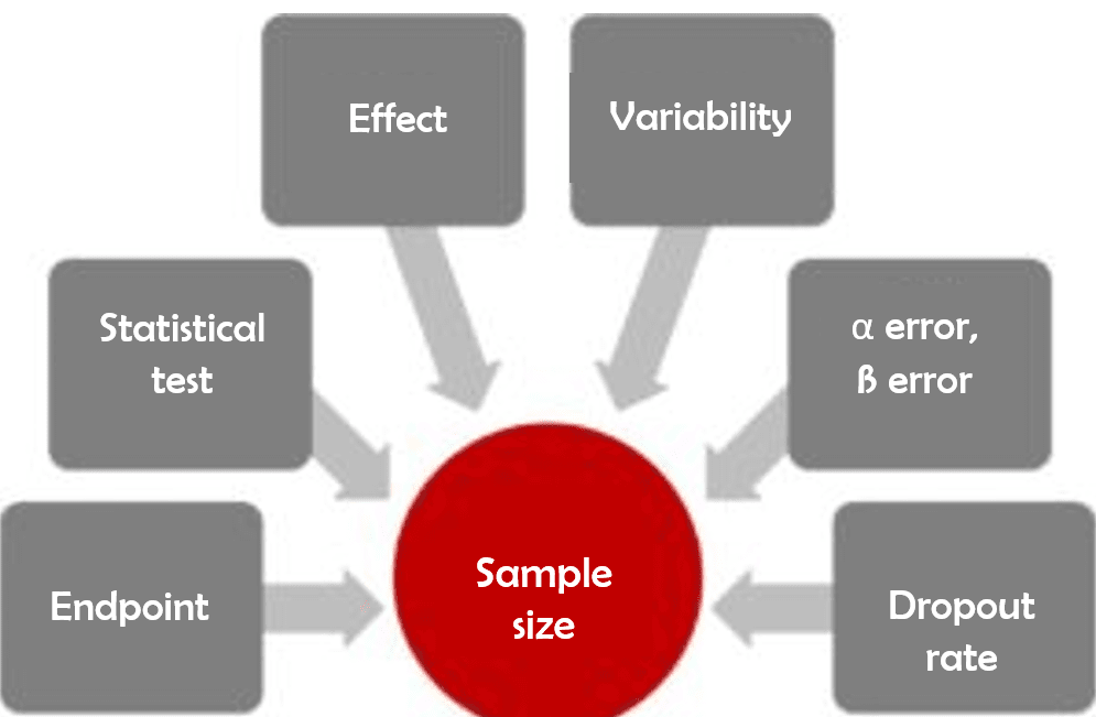
As this diagram shows, the final sample size is determined by several interconnected factors, including the expected effect, data variability, and the desired error rates.

Let's look at each of these in turn.

The Significance Level ( $α$ )
This is the threshold for declaring a result "statistically significant," representing the acceptable risk of a Type I error (false positive). It is almost universally set at $α = 0.05$ (for a two-sided test). A stricter (lower) $α$ demands stronger evidence, which in turn requires a larger sample size.
The Statistical Power ( $1 - β$ )
This is the desired probability of detecting a true effect, as we just discussed. For most Phase III trials, the power is conventionally set at 80% or 90%. A higher desired power means you want more certainty that you won't miss a real effect, which requires a larger sample size.
The Effect Size ( $Δ$ )
This is the magnitude of the difference between the treatment and control groups that the trial is designed to detect. This should be the minimum clinically important difference—the smallest effect that would be considered meaningful to patients and clinicians. For example, is a new blood pressure drug that lowers systolic pressure by an average of 2 mmHg more than the standard considered useful? What about 10 mmHg? The smaller the effect size you are trying to detect, the larger the sample size you will need. Detecting a subtle difference requires much more data than detecting a dramatic one.
The Variability of the Outcome ( $σ$ )
This refers to the spread or "noise" in the outcome measure, typically represented by the standard deviation. If an outcome (like blood pressure) varies a lot among individuals, it creates more statistical noise. To see a clear signal (the treatment effect) through this noise, you need a larger sample size. Estimates for variability often come from previous studies or pilot data.

The following image provides the classic visual representation of how these concepts fit together.

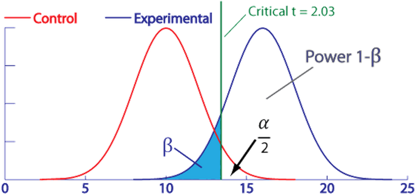
This graph illustrates the sampling distributions for a null hypothesis (Control, red) and an alternative hypothesis (Experimental, blue). The significance level $\alpha$ is the area in the tail of the null distribution beyond the critical value. The probability of a Type II error, $\beta$, is the area under the alternative distribution that falls short of this critical value. The power, $1-\beta$, is the remaining area under the alternative distribution, representing the probability of correctly detecting the effect.

The interplay between these four factors is fundamental. The following video provides excellent concrete examples of how changing each one affects a study's power.

Sample Size and Power: Fundamentals Part 1

This lecture from an NIH course provides a practical demonstration of how the core components of a sample size calculation are related.

Please watch the segment from this point in the video. The speaker walks through a list of the key elements and then gives numerical examples showing what happens to power when you change the standard deviation, the significance level, the effect size, or the sample size itself.

From Ingredients to a Final Number

While you won't be expected to perform these calculations by hand, it is useful to see how these elements combine. For a simple comparison of means between two groups, the formula for the sample size per group ( $n$ ) involves all four ingredients. A common formula looks something like this:

n = \frac{( z _{1 - α /2} + z _{1 - β} ) ^{2} σ ^{2}}{Δ ^{2}}

Where:

$z_{1 - α /2}$ and $z_{1 - β}$ are values from the standard normal distribution that correspond to the chosen $α$ and $β$ .
$σ^{2}$ is the variance (the square of the standard deviation).
$Δ^{2}$ is the square of the effect size.

Looking at this formula reinforces the relationships we've discussed:

The effect size ( $Δ$ ) is in the denominator. A smaller effect size leads to a much larger required sample size.
The variability ( $σ$ ) is in the numerator. Higher variability leads to a larger required sample size.
Choosing a stricter $α$ or higher power ( $1 - β$ ) increases the $z$ -values, also leading to a larger sample size.

A Crucial Practical Adjustment: Dropouts

The calculated sample size, $n$ , is the number of participants you need to complete the study and be included in the final analysis. However, in the real world, participants may drop out for various reasons. To ensure the study remains adequately powered, the initial number of enrolled participants must be inflated to account for this expected attrition.

The correct way to adjust for a dropout rate ( $d$ ) is:

N_{enrolled} = \frac{N _{required}}{1 - d}

For example, if you calculate that you need 400 participants to complete the study and you anticipate a 20% dropout rate, you must enroll $400/ (1 - 0.20) = 400/0.80 = 500$ participants. A common mistake is to simply add 20% (which would be 480), underestimating the number needed.

The following resource provides a concise explanation of this adjustment.

Statistical Sample Size Calculations for Clinical Trials

This is the final section of the blog post we viewed earlier.

Please read the short section titled Accounting for dropouts. It explains the rationale and provides the correct formula for this essential adjustment.

Conclusion

In this lesson, we have unpacked the critical concepts of statistical power and sample size. Designing a study that is large enough, but not too large, is fundamental to conducting ethical and efficient clinical research.

Here are the key takeaways:

Sample size calculation is a mandatory step in trial design to ensure scientific validity and ethical conduct, preventing underpowered or overpowered studies.
Statistical power is the probability ( $1 - β$ ) of a study correctly detecting a true treatment effect, thereby avoiding a false negative (Type II error).
The required sample size is determined by a trade-off between four key factors: the significance level ( $α$ ), the desired power ( $1 - β$ ), the expected effect size ( $Δ$ ), and the outcome variability ( $σ$ ).
A smaller effect size, higher variability, stricter significance level, or higher desired power will all increase the required sample size.
The calculated sample size must be inflated to account for the expected rate of participant dropouts.

Now that we understand how to plan for the right number of participants, and what to do about those who might drop out, our next lesson will address a related question: once the data is collected, how do we handle the analysis when some participants didn't follow the protocol perfectly or dropped out? We will explore the crucial distinction between intention-to-treat and per-protocol analysis principles.