Welcome back. The previous lesson compared the tiny MoE and dense checkpoints using held-out loss, total parameters, and active parameters. That comparison did not tell you how the MoE uses its experts. Here you will inspect routing on the same held-out split, grouped by the synthetic dataset’s token groups. The aim is a measurable statement—such as “group A selects experts 0 and 1 more often than group B”—rather than an unsupported claim that an expert has learned a particular skill.
What would specialization look like?
A router makes a decision for each token representation at each MoE layer. If tokens in different predefined groups consistently receive different expert selections, their group-conditioned routing distributions will differ. Overall expert utilization cannot reveal this by itself: every expert could receive an equal share of tokens globally while serving quite different mixtures of groups.
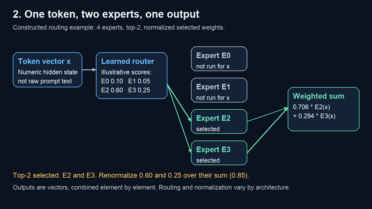
The distinction matters for top-two routing. In the image, E2 and E3 are both selected, even though their scores and final combination weights differ. A count of selected experts answers “where were these tokens sent?” It does not answer “which output had greater weight?”
Before measuring the tiny model, read an empirical example in OpenMoE: An Early Effort on Open Mixture-of-Experts Language Models. Its findings are useful precisely because apparent specialization changes with the grouping used.
OpenMoE: An Early Effort on Open Mixture-of-Experts Language Models
Read Section 4.1 to see how routing patterns differ when tokens are grouped by domain, language, task, position, or token ID. Then use Section 4.2 to examine the authors' interpretation of token-level patterns.
In Section 4.1, "What are the Experts Specializing in?", read the routing analysis from the opening paragraph through the final sentence about token-ID routing variation. In Section 4.2, "Token Specialization Study", look at Table 9 and read the first interpretation beneath it; stop before the paragraph beginning "When did the model learn the specialization?" Focus on why a pattern attributed to a domain might instead reflect the token IDs common in that domain.
The OpenMoE results are observations about that model and those data, not a rule that all routers ignore context. They establish a useful standard for your experiment: name the grouping variable before interpreting the pattern. In a synthetic dataset, a token group is known by construction. That makes it a clean variable to measure, but a preference for a group still does not prove what an expert computes.
Turn routing decisions into a conditional distribution
Choose one MoE layer and a fixed, held-out set of valid input-token positions. Let be the synthetic group assigned to the input token representation being routed at position . This alignment is important in a next-token model: the routed input token and its prediction target occupy different roles. If your dataset supplies sequence-level rather than token-level groups, use those labels instead and state that choice.
Suppose the layer has experts and selects distinct experts per token. Define as the number of selected-expert slots assigned to expert by tokens in group . If valid tokens belong to that group and every token has selections, the row has assignments. The group-conditioned distribution is
Each row of sums to one. It describes the expert for a uniformly sampled selected slot from that group. By contrast, is the fraction of group tokens that selected expert ; for top-, those fractions sum to , not one. Both can be useful, but do not switch denominators between rows.
For a concrete top-two example, imagine eight held-out tokens in each of two groups and four experts:
| Group | E0 selections | E1 selections | E2 selections | E3 selections |
|---|---|---|---|---|
| A | 6 | 6 | 2 | 2 |
| B | 2 | 2 | 6 | 6 |
There are selected slots per group. Thus group A has distribution , while group B has . Summed across groups, each expert has eight assignments: global load is perfectly balanced, yet routing is group-dependent.
To express the size of that difference with one number, first calculate the overall selected-slot distribution
Then calculate each group’s total-variation distance from it:
A value of zero means that group’s observed expert mix matches the overall mix; larger values indicate greater separation. In the example, the overall distribution is and . Report the conditional rows alongside this summary: the distance says how different, while the rows say which experts account for the difference.
Collect the measurements from the held-out checkpoint
Use the trained MoE checkpoint and the held-out split used for validation loss. Put the model in evaluation mode and disable any training-only router noise. For each MoE layer separately, collect the selected expert indices with shape [valid_tokens, k] and aligned group IDs with shape [valid_tokens]. Do not pool layers into one table: expert 0 in one layer is a different network from expert 0 in another.
The following code starts after you have collected those two tensors. Adapt the collection point to the supplied router scaffold rather than assuming a particular model-return format.
import torch

def group_routing_stats(expert_ids, group_ids, num_groups, num_experts):
    """
    expert_ids: [T, k] selected expert indices for valid input tokens
    group_ids:  [T] integer group labels in [0, num_groups)
    """
    if expert_ids.ndim != 2 or group_ids.ndim != 1:
        raise ValueError("Expected [T, k] expert IDs and [T] group IDs")

    tokens, k = expert_ids.shape
    if group_ids.shape[0] != tokens:
        raise ValueError("Token and group counts do not match")
    if not torch.all((group_ids >= 0) & (group_ids < num_groups)):
        raise ValueError("A group ID is outside the declared range")
    if not torch.all((expert_ids >= 0) & (expert_ids < num_experts)):
        raise ValueError("An expert ID is outside the declared range")

    # Each (group, selected expert) pair contributes one assignment.
    pair_ids = group_ids[:, None] * num_experts + expert_ids
    counts = torch.bincount(
        pair_ids.reshape(-1),
        minlength=num_groups * num_experts,
    ).reshape(num_groups, num_experts)

    group_tokens = torch.bincount(group_ids, minlength=num_groups)
    expected_assignments = group_tokens * k
    if not torch.equal(counts.sum(dim=1), expected_assignments):
        raise AssertionError("Selected-slot counts do not match top-k")

    counts_f = counts.float()
    conditional = counts_f / counts_f.sum(dim=1, keepdim=True).clamp_min(1)
    overall = counts_f.sum(dim=0) / counts_f.sum().clamp_min(1)
    distance = 0.5 * (conditional - overall).abs().sum(dim=1)

    return group_tokens, counts, conditional, overall, distance
Exclude padding, ignored positions, and positions without a defined group before calling this function. Ensure the labels and indices refer to the same flattened token order. As a basic check, inspect a few aligned (input token, group ID, selected experts) records from the held-out loader before trusting an aggregate table. If a group has zero held-out tokens, its computed zero row is a placeholder, not an estimated distribution; omit it from interpretation.
If your implementation limits expert capacity, decide which event you are measuring:
- Selected routing records the router’s top- choices before overflow. The code above measures this.
- Executed routing records contributions that actually reached experts after capacity decisions.
These can differ substantially for an overloaded group. Keep separate counts for dropped assignments by group and expert if capacity is active; never silently describe selected assignments as processed tokens. Likewise, gate weights are a different measurement from selection counts. You may report them additionally, but label whether they are full-softmax or renormalized top- weights.
Allow roughly 15 minutes for extraction and alignment checks, and another 5 for the tables and interpretation. The numerical example above provides a useful sanity check for the counting convention before using checkpoint data.
Interpret the pattern without mistaking it for a mechanism
A useful report has one conditional-routing table per layer, with group token counts, an overall expert row, and beside each group. State the checkpoint, held-out split, group definition, top-, and whether the table describes selected or executed routing. Small groups deserve caution: a striking row based on very few tokens is less persuasive than a similar pattern repeated across many held-out tokens.
Three comparisons make the interpretation sharper.
First, compare conditional routing with overall load. If one expert receives nearly everything from every group, the table shows global concentration, not meaningful group separation. If overall load is balanced but conditional rows differ, you have evidence of group-associated routing, as in the numerical example.
Second, inspect what the synthetic groups contain. If each group consists of disjoint token IDs, group association might be largely token-ID preference. If the same token ID can occur with different group labels or contexts, compare its routing within those contexts. You can also check whether groups differ systematically by sequence position. These checks distinguish a measured association from a premature story about semantic specialization.
Third, keep selection separate from usefulness. Conditional routing shows that the router sends groups to different experts; it does not establish that those experts improve predictions for those groups. A balanced auxiliary loss also does not force the conditional rows to be identical—it controls workload, not the interpretation of an expert’s contribution.
The core measurement is : expert-selection frequencies conditioned on a declared held-out token group, with a top- denominator that matches what you counted. Read those rows alongside global load, sample sizes, and any dropped-assignment counts. A distinct pattern supports a claim about routing association, not yet a claim about predictive benefit. The next lesson tests that stronger claim by measuring what happens to held-out loss when an apparent specialist’s contribution is removed.