Welcome back. Earlier in the course, you established how routing selects experts, how sparse dispatch works, and why total parameters differ from the parameters active for one token. The short training run in this module gives you an MoE checkpoint to evaluate. This lesson puts it beside the supplied dense baseline: you will account for both models’ parameters, measure validation loss on the same tokens, and interpret what an approximately matched-active-compute comparison can—and cannot—show.
What is being matched?
A useful dense baseline does not try to match the MoE’s total parameter count. Most MoE experts are idle for any particular token, whereas a dense feed-forward network uses its weights for every token. Instead, the supplied baseline is designed to be approximately matched in active computation: the work done along a token’s forward path is similar, even though the MoE stores more weights.
Start with the accounting distinction in Sebastian Raschka’s Why MoE Models Have Fewer Active Parameters.
Why MoE models have fewer active parameters
Read the parameter-count example and the discussion of active parameters as a compute proxy. They give you the conventions needed to label your comparison accurately.
In “A small parameter-count example,” read the worked count, beginning with the shared-parameter assumption and ending with why shared components change the ratio. Continue past the paragraph beginning “The same accounting applies across all MoE layers” to “Active parameters are a proxy for compute”; read the compute discussion. Focus on why an active-parameter count is useful but does not establish exact FLOPs or runtime.
Make the counting convention explicit before comparing checkpoints. Let count each unique shared parameter once, including embeddings, attention, normalization, any dense layers, and the output head. Let be the router parameters in MoE layer , and the parameters of its expert . Then
For a token , let contain the distinct experts it actually uses in layer . Its active count under this convention is
This includes the router, which scores experts for the token. Count tied weights only once in both totals. If all experts in a layer have the same size, routing selects a fixed number, and no contributions are dropped, the active count is constant across tokens. Otherwise, report a mean over validation tokens and state why it varies. A batch touching every expert does not make every expert active for each token.
Consider a small, illustrative single-layer comparison. Both models have shared parameters and hidden width . The MoE has four experts, selects two per token, and has a -by- router without bias. Each expert is a two-linear-layer feed-forward network of intermediate width , with a bias on each linear layer. Its parameter count is
A dense baseline uses one otherwise comparable feed-forward network of intermediate width . It has feed-forward parameters—exactly twice the count of one expert in this example.
| Illustrative model | Total parameters | Active parameters per token |
|---|---|---|
| Dense baseline | 56,912 | 56,912 |
| Four-expert, top-two MoE | 73,920 | 56,992 |
The MoE stores four expert networks but evaluates two for a token. The 80-parameter difference in active counts is its router. This is a close parameter-path match, not a proof of identical arithmetic: routing, the two separate expert evaluations, and their combination add work. For the supplied models, use their actual module sizes rather than these illustrative figures.
Read a published comparison without overreading it
The Switch Transformer comparison provides a larger-scale example of why dense and sparse models are often paired by computation rather than stored parameter count. In Section 5.6 of Fedus, Zoph, and Shazeer’s Scaling to Trillion Parameter Models with Simple and Efficient Sparsity, Table 9 places dense T5 and sparse Switch designs side by side.
[PDF] Scaling to Trillion Parameter Models with Simple and Efficient Sparsity
Read Section 5.6 and Table 9 to see how the authors report parameters, FLOPs per sequence, and model quality together. Treat it as a comparison design, not as a predicted result for your small experiment.
In Section 5.6, “Towards Trillion Parameter Models,” near printed p. 21, begin with the paragraph starting “Combining expert, model and data parallelism.” Read through Table 9, including both parts of the table. Compare the T5-Base/Switch-Base rows and the T5-Large/Switch-Large rows in the parameters and FLOPs columns, then locate the columns labeled “Neg. Log Perp.” for the quality results.
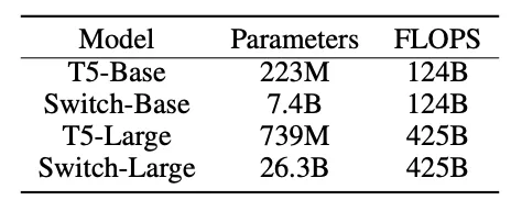
Table 9 rounds parameter totals, while the image displays more precise totals for these models. The important comparison is the same in both: total stored parameters differ greatly within each FLOP-matched pair. Table 9 also reports negative log perplexity, not your experiment’s validation-loss column. When interpreting that published metric, higher (less negative) is better; for the mean cross-entropy loss you will report below, lower is better. Keep the metric name attached to every number rather than placing unlike measures in one unlabeled “quality” column.
Even a published FLOP match leaves practical differences. Sparse routing and expert dispatch have costs; batch sizes and kernels affect efficiency. Conversely, matching active parameters is only a first approximation to a FLOP match. Your small experiment can test validation quality under its controlled setup. It cannot establish that either architecture is universally faster or better at scale.
Evaluate the two checkpoints on identical validation tokens
Use the held-out split from the short training experiment for both checkpoints. If the supplied baseline is already defined, retain its architecture rather than adjusting it after seeing validation loss. Verify that it uses the same tokenization, prediction task, and validation examples as the MoE.
For a next-token decoder, report mean negative log-likelihood per valid target token:
where is the set of non-ignored validation targets. Averaging the sum of token losses is important: an unweighted average of batch means gives a short final batch the same influence as a full batch. Exclude padding or ignored targets from both the numerator and denominator.
The following PyTorch pattern assumes the validation loader supplies already-aligned (inputs, targets) pairs and the model returns logits of shape [batch, time, vocab]. Adapt the logits-extraction line if the supplied scaffold returns a dictionary or a tuple; do not shift targets a second time if the dataset has already done so.
import torch
import torch.nn.functional as F

def validation_nll(model, validation_loader, device, ignore_id=-100):
    was_training = model.training
    model.eval()
    loss_total = 0.0
    token_total = 0

    with torch.inference_mode():
        for inputs, targets in validation_loader:
            inputs = inputs.to(device)
            targets = targets.to(device)

            logits = model(inputs)  # Adapt if the model returns more than logits.
            vocab_size = logits.shape[-1]
            loss_sum = F.cross_entropy(
                logits.reshape(-1, vocab_size),
                targets.reshape(-1),
                ignore_index=ignore_id,
                reduction="sum",
            )
            loss_total += loss_sum.item()
            token_total += targets.ne(ignore_id).sum().item()

    model.train(was_training)
    if token_total == 0:
        raise ValueError("Validation set has no non-ignored targets")
    return loss_total / token_total
Run this once for each final checkpoint on the same validation loader. Use inference mode and eval() so dropout does not turn the comparison into a comparison of random training-time passes. If MoE training used an auxiliary balancing loss or router z-loss, report the next-token validation NLL alone here: adding those training regularizers to one model’s reported value would make the quality columns incomparable. Check how the supplied code handles overflow; dropped expert contributions can change both effective computation and quality, even when the configured top- is unchanged.
For the training-side comparison, record the number of optimizer steps and the number of training target tokens seen. Equal steps are not an equal-data comparison if batch sizes or token counts differ. Keep the validation split fixed; if you run multiple seeds, report the per-seed results or their spread rather than selecting only the most favorable run.
Produce an auditable report
Count parameters from the checkpoint’s unique parameter tensors, including parameters that did not receive gradients on a particular batch. In PyTorch, sum(p.numel() for p in model.parameters()) gives the stored model-parameter total; check tied-weight handling in the supplied model so you do not count a shared embedding/output tensor twice. Partition the MoE total into shared, router, and expert counts to compute its active figure. For an equal-size, top- layer without dropped contributions, that layer contributes its router parameters plus expert parameter sets to the active count—not all its experts.
Place the measured values in one table. A compact report has this form; the entries below are fields to fill from the supplied runs, not results.
| Model | Validation NLL (nats/valid token) | Total parameters | Active parameters/token |
|---|---|---|---|
| Supplied dense baseline | measured value | checkpoint count | same as total |
| Tiny MoE | measured value | checkpoint count | shared + routers + selected experts |
Below the table, state the expert count, top-, how you treated tied weights and shared layers, and whether capacity drops occurred. State the training-token budget and validation-token count as well. If you have measured FLOPs for the same input shape, give them separately; do not label active parameters as FLOPs.
Interpret the loss difference as
A negative value means the MoE achieved lower held-out NLL in this run. The conclusion should also retain the cost qualifier: at approximately matched active compute, with the MoE’s stated total parameter count. A lower MoE loss does not show that its extra experts are semantically specialized, and a higher loss does not show sparse routing is inherently ineffective. Both outcomes can depend on training duration, routing balance, dropped assignments, and the small dataset.
The comparison has two inseparable parts: validation NLL measures predictive quality, while total and active parameter counts describe different resource demands. Matching the active path makes a dense baseline informative, but measured FLOPs and runtime remain distinct questions. Next, you will inspect held-out routing by token group to see whether the MoE’s extra stored capacity is associated with observable expert specialization.