Decision Trees: Classification & Regression

Part 1: The Anatomy of a Decision Tree

At its core, a decision tree is a flowchart-like structure. You start at the top (the root) and follow a path down by answering a series of yes/no questions about your data features until you reach a final outcome at a leaf.

There are two main types of decision trees, which directly correspond to the two main types of supervised learning tasks you've seen:

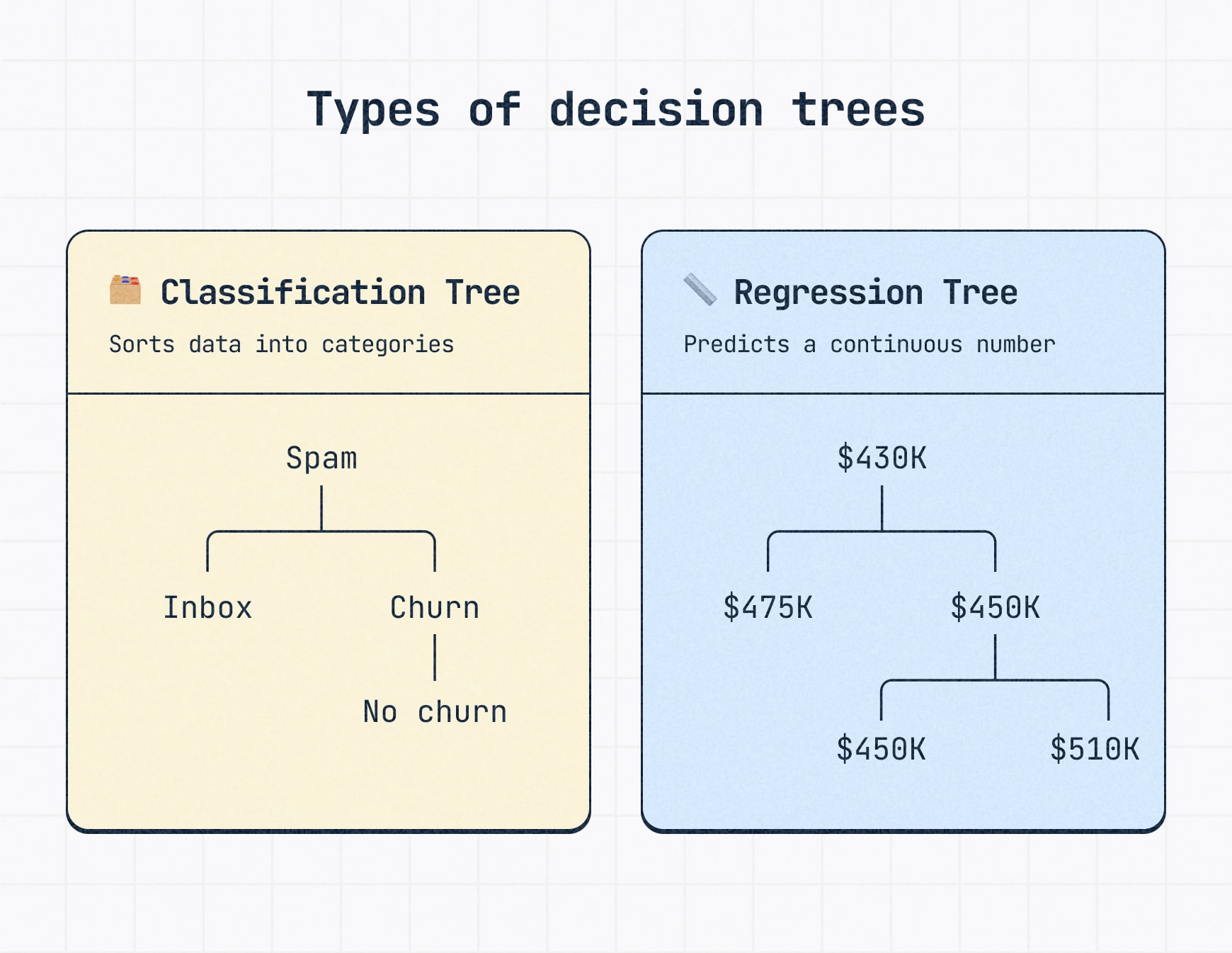
To get a feel for how these trees work in practice, let's start with a video that clearly explains the basic concepts and terminology.

As the video explained, every decision tree consists of:

• Root Node: The single top-most node, which represents the entire dataset and the first question you ask.
• Internal Nodes (or Branches): Nodes that represent a question or a "test" on a feature. They have arrows pointing to them and arrows pointing away from them.
• Leaf Nodes: The terminal nodes of the tree where the final prediction (a class label or a numeric value) is made. They have arrows pointing to them but none pointing away.

Interpreting a tree is as simple as starting at the root and traversing the path based on the answers to the questions at each node until you reach a leaf. Each path from the root to a leaf represents a specific decision rule.

Part 2: Building a Tree - The Core Idea

How does an algorithm decide which questions to ask, in what order, and what thresholds to use? The process of building a tree is conceptually straightforward and is often done using an algorithm called CART (Classification and Regression Trees).

The core idea is to perform a series of splits that make the resulting groups of data more "pure" or homogeneous.

• For a classification tree, a node is pure if it contains samples from only one class.
• For a regression tree, a node is "pure" (or homogeneous) if the samples it contains have very similar numerical values (i.e., low variance).

The algorithm takes a top-down, greedy approach. "Top-down" means it starts at the root with all the data and recursively splits it. "Greedy" means that at each step, it chooses the single best split possible at that moment to achieve the most significant immediate increase in purity, without looking ahead to see if a different split now might lead to an even better overall tree later.

To decide which split is "best," we need a way to numerically measure the purity of a node. For classification, a common metric is the Gini Impurity.

For now, you only need to know that a lower Gini Impurity score is better. The algorithm calculates the Gini score for every possible split on every feature and chooses the split that results in the largest reduction in Gini impurity. We will dive into the exact formula for Gini impurity in our next lesson.

For regression trees, the logic is similar. Instead of maximizing purity, the goal is to find splits that minimize the error in the child nodes. A common metric for this is the Sum of Squared Residuals (SSR) or Mean Squared Error (MSE). The prediction made at a leaf is simply the average of the target values of all the training samples that end up in that leaf.

Part 3: Building a Decision Tree in Python

Now let's move from theory to practice. We will use the scikit-learn library, which provides easy-to-use implementations for both classification and regression trees.

The key classes are DecisionTreeClassifier and DecisionTreeRegressor. A crucial parameter for both is max_depth. This parameter limits how many "layers" of questions the tree can ask. It's one of the most common ways to control the complexity of the tree and prevent overfitting—a situation where the model learns the training data perfectly but fails to generalize to new, unseen data.

Let's walk through the key steps for building a classification tree from that resource:

1. Import and Instantiate: First, you import the class and create an instance of the model. You can set hyperparameters like max_depth here.

   from sklearn.tree import DecisionTreeClassifier
   
   # Instantiate the classifier with a maximum depth of 5
   # and require at least 10 samples in a leaf node.
   clf = DecisionTreeClassifier(max_depth=5, min_samples_leaf=10, random_state=42)
   

2. Fit the Model: Train the model on your training data.

   # Assume X_train and y_train are your training features and labels
   clf.fit(X_train, y_train)
   

3. Visualize the Tree: This is the most powerful step for interpretation. Scikit-learn's plot_tree function makes it easy.

   from sklearn.tree import plot_tree
   import matplotlib.pyplot as plt
   
   plt.figure(figsize=(20, 10))
   plot_tree(clf, 
             feature_names=X_train.columns, 
             class_names=['Class_0', 'Class_1'], 
             filled=True, 
             rounded=True)
   plt.show()
   

The process for a regression tree is almost identical; you just use DecisionTreeRegressor instead and the criteria shown in the nodes will be based on MSE instead of Gini impurity.

Conclusion

In this lesson, you've learned the fundamentals of decision trees, one of the most interpretable and foundational models in machine learning. You can now explain what a tree is, how it works for both classification and regression, and how to build and interpret one yourself.

Key Takeaways:

• Decision trees make predictions by asking a series of if-then-else questions on features.
• Classification trees predict a class label at the leaf nodes, while regression trees predict a continuous value (typically the average of the samples in that leaf).
• Trees are built using a greedy, top-down approach, where each split is chosen to maximize the homogeneity (or "purity") of the resulting child nodes.
• For classification, purity is often measured by Gini Impurity. For regression, prediction error is often measured by Mean Squared Error (MSE).
• You can easily build, train, and visualize trees in Python using scikit-learn, which is crucial for interpretation. Key parameters like max_depth help control complexity and prevent overfitting.

Preview of the Next Lesson:
We've mentioned that the algorithm chooses the "best" split by measuring impurity. But how does that work mathematically? In our next lesson, we will lift the hood and explore the specific split criteria like Gini impurity and Information Gain, giving you the statistical foundation to understand exactly why the tree makes the decisions it does.