P-Values and Data-Driven Decisions

Hello! Welcome to your next lesson in the Statistical Inference and Estimation module.

In our last session, we established the crucial first step of hypothesis testing: formulating a clear question in the form of a null hypothesis ( $H_{0}$ ) and an alternative hypothesis ( $H_{a}$ ). We framed $H_{0}$ as the "status quo" or "no effect" assumption, and $H_{a}$ as the new claim we want to find evidence for.

Today, we move to the second step: answering that question. We will learn how to quantify the strength of evidence against the null hypothesis using a single, powerful number—the p-value. This will allow us to make a formal, data-driven decision: is the effect we observed in our sample strong enough to conclude it's real, or could it just be random chance?

Your learning outcome for this lesson is to calculate p-values from test statistics and use them to make data-driven decisions.

1. What is a P-value? The "Surprise" Index

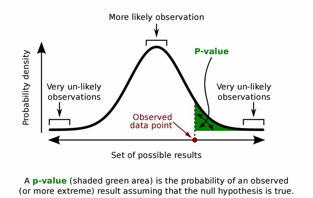
Imagine you're testing a new model and it shows a 2% accuracy improvement on your test set. The p-value answers a specific question:

"If the new model was actually no better than the old one (i.e., if the null hypothesis is true), what is the probability that we would see an improvement of 2% or even more, just by pure random luck?"

A small p-value indicates that your observed result would be very surprising if the null hypothesis were true. This "surprise" is evidence against the null hypothesis.

Small P-value: "Wow, this result is really unlikely if there's no real effect. Maybe there is a real effect after all."
Large P-value: "Well, a result like this is pretty common even when there's no real effect. I don't have enough evidence to say anything new."

P-value Illustration with Probability Density Function — This image illustrates the p-value. Assuming the null hypothesis is true, the curve shows the probability of all possible outcomes. Our observed data point falls in the tail. The p-value is the shaded area, representing the probability of getting a result as extreme as, or more extreme than, our observation.

Let's start by building a solid intuition for what a p-value represents and how it's calculated in a simple scenario.

How to calculate p-values

This StatQuest video with Josh Starmer provides an excellent, step-by-step introduction to the p-value using a simple coin-flipping experiment. It clearly breaks down the components that go into calculating it.

Watch from 0:51 to 9:20. Focus on how the p-value is a sum of three parts: the probability of your observation, the probability of equally rare observations, and the probability of rarer observations.

As the video highlights, the p-value isn't just the probability of your specific result; it's the probability of your result or anything more extreme. This is a fundamental point.

2. The Decision Rule: P-value vs. Significance Level ( $α$ )

So, how small does a p-value have to be for us to declare our result "surprising" enough to reject the null hypothesis? This is where the significance level, denoted by $α$ (alpha), comes in.

The significance level $α$ is a threshold we set before we conduct our test. It represents the risk we're willing to take of making a Type I error—that is, rejecting the null hypothesis when it's actually true. The most common value for $α$ is 0.05 (or 5%).

The decision rule is straightforward:

If p-value ≤ $α$ , we reject the null hypothesis ( $H_{0}$ ). We conclude that the result is statistically significant.
If p-value > $α$ , we fail to reject the null hypothesis ( $H_{0}$ ). The result is not statistically significant.

Important Note: We "fail to reject" $H_{0}$ , we don't "accept" it. This is like a jury finding a defendant "not guilty" rather than "innocent." We're not proving the null hypothesis is true; we're just saying we don't have enough evidence to discard it.

The following text provides a concise summary of this decision-making framework.

S.3.2 Hypothesis Testing (P-Value Approach) | STAT ONLINE

This page from Penn State's STAT ONLINE course clearly outlines the P-value approach and the four steps involved in any hypothesis test, focusing on the comparison between the p-value and alpha.

Read the introductory paragraphs and the list of four steps. This will formalize the decision-making process we've just discussed.

3. Calculating the P-value from a Test Statistic

In practice, we rarely count discrete outcomes like with coin flips. For continuous data (like model accuracy, user engagement time, or sales figures), we follow this process:

Calculate a Test Statistic: We first summarize our sample data into a single number called a test statistic (e.g., a z-statistic or t-statistic). This statistic measures how many standard deviations our sample result is from the value stated in the null hypothesis.
Find the P-value: We then use the known probability distribution of that test statistic (like the Normal or t-distribution) to find the probability of observing a value as extreme or more extreme. This probability is the p-value.

Let's see how this works for continuous data.

How to calculate p-values

We'll return to the StatQuest video, which now extends the concept from coin flips to continuous data (height measurements). This is a great visual for understanding how the p-value corresponds to an area under a distribution curve.

Watch from 12:12 to 20:02. Notice how 'more extreme' now means 'further away from the mean' on the distribution.

Now, let's walk through a complete, practical example that ties everything together: the hypotheses, the test statistic, the p-value calculation, and the final decision.

Calculating a P-value given a z statistic | AP Statistics | Khan Academy

This Khan Academy video provides a perfect, concise example. It starts with a problem, states the hypotheses, uses a given Z-statistic to find the p-value from a table, and makes a conclusion based on the significance level.

Watch the entire video. This demonstrates the exact workflow you'll use to solve hypothesis testing problems.

One-Tailed vs. Two-Tailed Tests

Remember from our last lesson that your alternative hypothesis ( $H_{a}$ ) can be directional ( $>$ or $<$ ) or non-directional ( $\neq =$ ). This determines how you calculate the p-value.

P-Value Approach in Hypothesis Testing — This diagram shows how the p-value is calculated for different tests. For a **right-tailed test** ($H_a: \mu > \mu_0$), the p-value is the area in the right tail. For a **left-tailed test** ($H_a: \mu < \mu_0$), it's the area in the left tail. For a **two-tailed test** ($H_a: \mu \neq \mu_0$), you consider extreme results in both directions, so the p-value is the sum of the areas in both tails.

The STAT ONLINE resource you looked at earlier has excellent visual examples of this.

S.3.2 Hypothesis Testing (P-Value Approach) | STAT ONLINE

Let's revisit the STAT ONLINE page to see clear, side-by-side examples of calculating p-values for right-tailed, left-tailed, and two-tailed tests.

Read the three examples titled 'Mean GPA', one for each test type (Right Tailed, Left Tailed, Two-Tailed). Pay close attention to how the calculation changes for the two-tailed test (the p-value is doubled).

The final segment of the StatQuest video also offers a practical warning about using one-sided tests, which is a valuable piece of advice. It explains why a two-sided test is often safer because it can detect an unexpected effect in the opposite direction.

Test your understanding!

You are A/B testing a new recommendation algorithm. Your null hypothesis is that the new algorithm has no effect on user watch time ( $H_{0} : μ_{n e w} = μ_{o l d}$ ). Your alternative is that it has a different effect ( $H_{a} : μ_{n e w} \neq = μ_{o l d}$ ). You set your significance level $α = 0.05$ .

After running the experiment, you calculate a test statistic that corresponds to a p-value of 0.03.

Is this a one-tailed or two-tailed test?
Based on the p-value, what is your conclusion about the null hypothesis?
Is the result statistically significant?
What if the p-value had been 0.12 instead? What would your conclusion be?

Show answer

This is a two-tailed test, because the alternative hypothesis is $\neq =$ (testing for a difference in either direction).
Since the p-value (0.03) is less than or equal to $α$ (0.05), you reject the null hypothesis.
Yes, the result is statistically significant. You have evidence to conclude that the new algorithm has a different effect on user watch time.
If the p-value were 0.12, it would be greater than $α$ (0.05). In that case, you would fail to reject the null hypothesis. The result would not be statistically significant, and you would conclude that you don't have enough evidence to say the new algorithm is any different from the old one.

4. P-values in Machine Learning Practice

This entire framework is directly applicable to your goal of justifying ML models. P-values are not just for academic statistics; they are used in ML to make concrete decisions. Two common use cases are:

Assessing Feature Importance: In models like linear and logistic regression, each feature (or coefficient) has an associated p-value. This tests the null hypothesis that the feature has no effect on the outcome. A small p-value suggests the feature is a statistically significant predictor.
Comparing Model Performance: When you compare Model A to Model B, you can perform a statistical test where the null hypothesis is "there is no difference in performance between the models." A small p-value gives you evidence to claim your new model is genuinely better (or different).

The following article shows how to implement these ideas in Python.

Mastering P-values in Machine Learning

This article from Towards Data Science, 'Mastering P-values in Machine Learning', provides excellent context and code examples for using p-values in common ML tasks.

Read the sections 'P-values for Linear Regression Coefficients', 'P-values for Logistic Regression Coefficients', and 'P-values for comparing... Models'. You don't need to run the code, but focus on how the hypotheses are set up and how the resulting p-values are interpreted to make decisions about features and models.

Conclusion

You have now learned the complete, fundamental logic of hypothesis testing. You started by framing a question with null and alternative hypotheses, and today you learned how to answer it using a p-value. This process allows you to move from simply observing a difference to making a statistically-backed claim about whether that difference is meaningful.

Key Takeaways:

The p-value is the probability of observing a result as or more extreme than your sample result, assuming the null hypothesis is true. It's a measure of how surprising your data is.
The significance level ( $α$ ) is your pre-defined threshold for "surprise," typically 0.05.
The decision rule is simple: if p-value $\leq α$ , you reject $H_{0}$ and the result is statistically significant.
The calculation of the p-value depends on your test statistic and whether you are conducting a one-tailed or two-tailed test.
In machine learning, p-values are used to assess feature importance and to formally compare the performance of different models.

Preview of the Next Lesson:

So far, we have been working with test statistics and population parameters that are assumed or given. But in the real world, how do we come up with the initial estimates for these parameters in the first place? In our next lesson, we will explore our first formal estimation technique: the method of moments. You will learn how to use sample data to estimate the parameters of a probability distribution.

Recommended resources