Calculating Attention Scores

1. From Embeddings to Q, K, and V

In the last lesson, we treated Queries, Keys, and Values as abstract concepts. In a real Transformer, these are concrete vectors that are created from the initial word embeddings. How does the model generate a query (what to look for) and a key (what I have) from the same initial word?

The answer is through learned linear projections. The model uses three distinct weight matrices, which we'll call $W_Q$, $W_K$, and $W_V$. Each input embedding vector ($x$) is multiplied by each of these matrices to produce its corresponding query ($q$), key ($k$), and value ($v$) vectors.

The crucial point is that the matrices $W_Q$, $W_K$, and $W_V$ contain parameters that are learned during the training process. This allows the model to learn the optimal way to transform an input embedding for its three different roles:

• Querying: What features of an embedding are useful for finding related information?
• Being Queried (Key): What features should be advertised to attract relevant queries?
• Contributing (Value): What information should be passed along when attention is paid?

To get a deeper intuition for this, let's watch a video that explains the role of these matrices.

For a detailed, step-by-step breakdown of this projection, the following reading is excellent.

2. Calculating Attention Scores: Scaled Dot-Product

Once we have our Query and Key vectors, we need to calculate a similarity score between them. As we discussed previously, the dot product is an efficient way to do this. For an entire sequence of $n$ tokens, we can compute all $n^2$ pairwise scores between every query and every key using a single matrix multiplication:

Here, $Q$ and $K$ are matrices where each row is a query or key vector, respectively. This operation leverages the power of GPUs and is a key reason for the efficiency of Transformers.

However, there's a subtle but critical problem. As the dimension of the key vectors ($d_k$) increases, the variance of the dot products also increases. Larger dot product values can push the softmax function (our next step) into regions where its gradient is almost zero. This makes it very difficult for the model to learn effectively.

The solution, introduced in the original "Attention Is All You Need" paper, is simple and elegant: scale the scores. We divide the dot product scores by the square root of the dimension of the key vectors, $\sqrt{d_k}$.

This scaling ensures that the scores have a more stable variance, regardless of the size of $d_k$, leading to more stable training.

Let's continue with the same article, which provides an excellent statistical justification for this scaling factor.

3. From Scores to Weights: The Softmax Function

Now that we have our scaled scores, the next step is to convert them into attention weights. These weights represent a probability distribution, indicating how much attention each token should pay to every other token in the sequence. As you know from the previous lesson, we use the softmax function for this.

The softmax function is applied to each row of the scaled score matrix.

The result is a matrix where each entry is between 0 and 1, and each row sums to 1. An entry at position $(i,j)$ in this matrix represents the amount of attention that token $i$ pays to token $j$.

The following video provides a fantastic visualization of this process.

4. The Full Picture: Scaled Dot-Product Attention

We have now assembled all the pieces. The final step is to use these attention weights to create the output. This is done by taking a weighted sum of the Value vectors.

The complete formula for Scaled Dot-Product Attention is:

This single, powerful equation encapsulates the entire process:

1. $Q{K}^T$: Compute dot product similarity scores between all queries and keys.
2. $\frac{\dots }{\sqrt{d_k}}$: Scale the scores for numerical stability.
3. $\text{softmax}(\dots )$: Normalize the scores into attention weights (a probability distribution).
4. $\dots V$: Multiply the weights by the Value matrix to get a weighted sum of the values.

The resulting matrix contains the new, contextually enriched representations for each token in the sequence.

The following image provides a great visual summary of this entire flow.

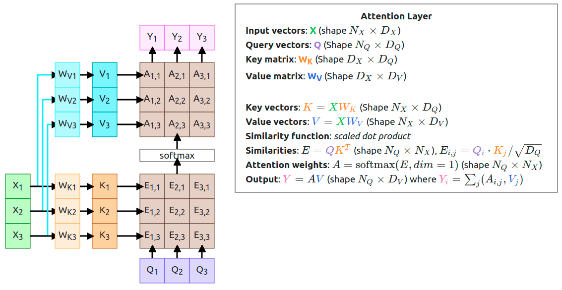
To see this entire process with concrete numbers, the last section of the article we've been reading provides a fantastic worked example.

Conclusion

In this lesson, we have demystified the calculation of attention scores, moving from the high-level intuition of the last session to the concrete matrix operations that are actually performed.

Key Takeaways:

• Projection is Key: Query, Key, and Value vectors are not inherent properties but are created by projecting input embeddings through three learned weight matrices: $W_Q$, $W_K$, and $W_V$.
• Scaled Dot-Product is the Core: The similarity score is calculated using a dot product, which is then scaled by $\sqrt{d_k}$ to ensure stable training.
• The Full Formula: The entire process is elegantly captured by the scaled dot-product attention formula: $\text{Attention}(Q,K,V)=\text{softmax}\left(\frac{Q{K}^T}{\sqrt{d_k}}\right)V$.
• Efficiency: These operations are primarily matrix multiplications, which are highly optimized on modern hardware like GPUs, making attention computationally feasible.

Preview of the Next Lesson:

The mechanism we learned today is a single "attention head." But what if a word needs to pay attention to different things for different reasons (e.g., attending to a subject for grammatical agreement and to an adjective for semantic meaning)? The solution is multi-head attention, where the model runs multiple attention heads in parallel, each learning different types of relationships. In our next lesson, we will explore this concept and see how it allows Transformers to capture a much richer set of dependencies.