Understanding Vanishing and Exploding Gradients in RNNs

1. The Root of the Problem: Backpropagation Through Time (BPTT)

To understand where things go wrong, we first need to recall how a neural network learns. It uses backpropagation to calculate the gradient of the loss function with respect to each weight. This gradient tells the optimizer how to adjust the weights to reduce the error.

In an RNN, the output at a given time step (e.g., the 10th word in a sequence) depends on computations from all previous time steps. Therefore, to calculate the gradient for a weight that was used in an early time step, the error signal must be propagated backward from the end of the sequence all the way to the beginning. This process is called Backpropagation Through Time (BPTT).

Let's read a short introduction to this concept.

As the article states, the key takeaway is that BPTT uses the chain rule to calculate gradients. This means the gradient at an early time step is the result of multiplying many smaller gradient terms together, one for each step back in time.

This chain of multiplications is the source of our problems.

2. Exploding and Vanishing Gradients: A Visual Intuition

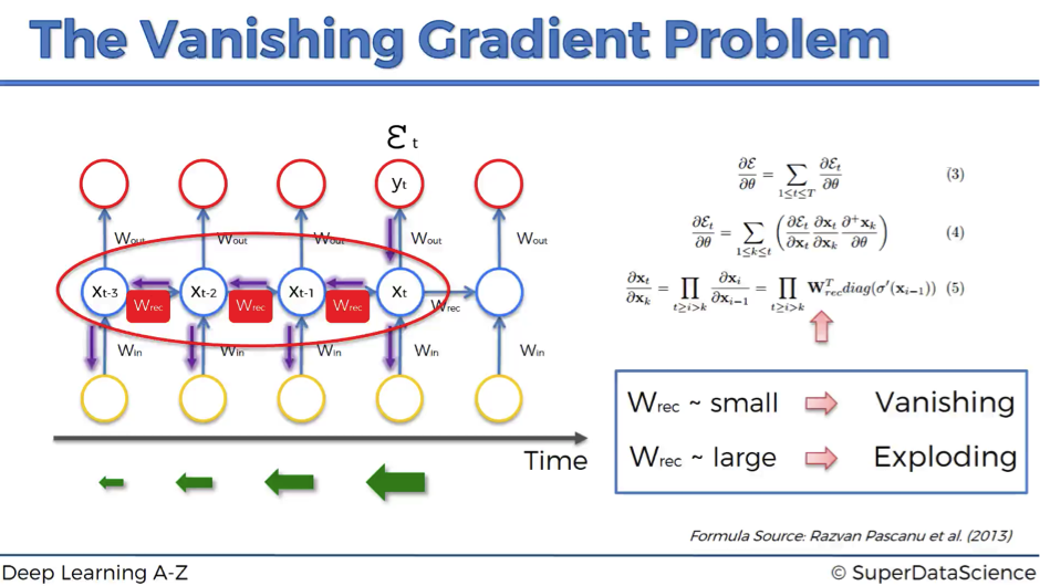
Depending on the values of the terms we are repeatedly multiplying, the final gradient signal can either grow exponentially until it's uselessly large (exploding gradients) or shrink exponentially until it's uselessly small (vanishing gradients).

The StatQuest video below gives a brilliant and simple visual intuition for both of these scenarios.

Let's formalize what you just saw:

• Exploding Gradients: Occurs when the gradients are repeatedly multiplied by numbers greater than 1. The gradient signal grows exponentially, resulting in huge weight updates. This makes the training process unstable, and you'll often see the loss function result in NaN (Not a Number) or Inf (Infinity) values.
• Vanishing Gradients: Occurs when the gradients are repeatedly multiplied by numbers less than 1. The gradient signal shrinks exponentially, becoming close to zero for early time steps. The network effectively stops learning from information seen long ago.

3. The Practical Consequence: Short-Term Memory

The exploding gradient problem is frustrating but easy to spot. The vanishing gradient problem is more insidious. The network might appear to be training fine, but it becomes incapable of learning long-range dependencies.

Imagine trying to predict the last word of this sentence:

"I grew up in France and I love the culture, the food, the art... I speak fluent _____."

To predict "French," the model needs to "remember" the word "France" from the beginning of the sentence. If the gradient signal from the end of the sentence has vanished by the time it gets back to the beginning, the weights that process "France" will not be updated properly to help with the prediction. The RNN effectively has short-term memory.

The following video provides an excellent walkthrough of this exact issue in a Natural Language Processing (NLP) context.

4. A Formal Look and a Simple Solution

So far, we have built a strong intuition. The core mathematical mechanism involves the repeated multiplication of the Jacobian matrix $\frac{\partial h_t}{\partial h_{t-1}}$, which is heavily influenced by the recurrent weight matrix $W_{hh}$ from our previous lesson.

The gradient of the loss $L$ at a late time step $T$ with respect to a hidden state at an early time step $t$ is a product:

If the norm of the terms in the product $\left(\frac{\partial h_k}{\partial h_{k-1}}\right)$ is consistently > 1, the overall gradient explodes. If it's consistently < 1, it vanishes.

While the vanishing gradient problem is harder to solve, there is a very common and effective technique for the exploding gradient problem.

As the article mentioned, gradient clipping is a simple and practical solution for exploding gradients. It works by setting a predefined threshold for the gradient's magnitude. If a gradient exceeds this threshold during backpropagation, it's "clipped" or scaled down to the maximum value. This prevents the massive, destabilizing weight updates.

Conclusion

In this lesson, we dissected a fundamental weakness of simple Recurrent Neural Networks. While powerful in theory, their reliance on backpropagation through time makes them susceptible to unstable gradients.

Key Takeaways:

• Backpropagation Through Time (BPTT): The process of training RNNs involves unrolling the network and propagating gradients through the entire sequence, which requires repeated multiplication via the chain rule.
• Vanishing Gradients: If recurrent weight matrices and activation function derivatives are small (norm < 1), the gradient signal shrinks exponentially, preventing the network from learning long-range dependencies. This results in a model with only "short-term memory."
• Exploding Gradients: If recurrent weight matrices are large (norm > 1), the gradient signal grows exponentially, leading to numerical instability (NaN values) and divergent training.
• Mitigation: Exploding gradients can be effectively handled using gradient clipping. The vanishing gradient problem is more difficult and required a fundamental change in the network's architecture.

Preview of the Next Lesson:

The vanishing gradient problem was a major obstacle in the history of deep learning. To solve it, researchers developed more sophisticated recurrent units. In our next lesson, we will explore the Long Short-Term Memory (LSTM) cell, an ingenious architecture that uses a system of "gates" to explicitly control the flow of information, allowing it to remember or forget information over long sequences and finally overcome the challenge of vanishing gradients.