Understanding LSTM Architecture and Vanishing Gradients

1. The Core Idea: A Separate Path for Memory

The brilliant insight behind LSTMs is to create a dedicated pathway for information to travel through time with minimal interference. This pathway is called the cell state. Think of it as an express conveyor belt or a data highway running through the entire sequence.

Information can flow along this cell state largely unchanged, which is the key to preserving gradients over long distances. The LSTM can then carefully add or remove information from this cell state using specialized neural networks called gates.

To get a high-level overview of this concept, let's watch a short segment from a video by StatQuest.

This separation is the foundation of the LSTM's power. Now, let's dive into the mechanics of how the cell state is controlled.

2. The Architecture of an LSTM Cell

An LSTM cell looks more complex than a simple RNN cell because it contains four interacting neural network layers instead of just one. These layers work together to implement the gates and update the cell state.

Let's begin with a fantastic article from Christopher Olah's blog, which provides an exceptionally clear, step-by-step walkthrough.

As the article explains, the LSTM cell uses three gates to protect and control the cell state:

1. Forget Gate: Decides what information to throw away.
2. Input Gate: Decides what new information to store.
3. Output Gate: Decides what to output as the hidden state.

Before we examine each gate, it's important to understand the two main activation functions used within them: sigmoid and tanh.

• Sigmoid ($\sigma$): This function squashes any real number into the range [0, 1]. It's perfect for a gate mechanism: a value of 0 means "let nothing through," while a value of 1 means "let everything through."
• Hyperbolic Tangent ($tanh$): This function squashes any real number into the range [-1, 1]. It's typically used to create new "candidate" values to be added to the cell state.

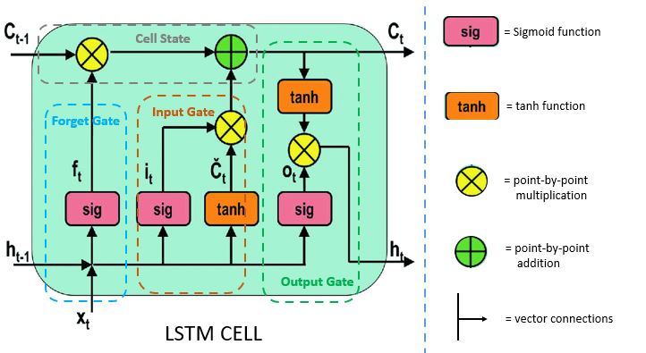
Now, let's walk through the LSTM cell, one gate at a time. The diagram below shows a detailed view of a single cell, which we will refer to as we break down each component.

Step 1: The Forget Gate

The first step is to decide what information to discard from the previous cell state ($C_{t-1}$). The forget gate takes the previous hidden state ($h_{t-1}$) and the current input ($x_t$) and passes them through a sigmoid layer. The output, $f_t$, is a vector with values between 0 and 1. This vector is then multiplied element-wise with the previous cell state.

The equation for the forget gate is:
$f_t=\sigma (W_f\cdot [h_{t-1},x_t]+b_f)$
Here, $[h_{t-1},x_t]$ represents the concatenation of the previous hidden state and the current input.

Step 2: The Input Gate

Next, the cell decides what new information to store. This is a two-part process:

1. The input gate layer (a sigmoid function) decides which values to update.
2. A tanh layer creates a vector of new candidate values, ${\tilde{C}}_t$, that could be added to the state.

These two parts are then multiplied to create the update.

The equations are:
$i_t=\sigma (W_i\cdot [h_{t-1},x_t]+b_i)$
${\tilde{C}}_t=\tanh (W_C\cdot [h_{t-1},x_t]+b_C)$

Step 3: Updating the Cell State

Now we can update the old cell state $C_{t-1}$ into the new cell state $C_t$. We multiply the old state by the forget gate's output, $f_t$, and then add the new candidate values scaled by the input gate, $i_t\ast {\tilde{C}}_t$.

$C_t=f_t\odot C_{t-1}+i_t\odot {\tilde{C}}_t$
The $\odot$ symbol denotes element-wise multiplication. This additive interaction is the most critical part of the LSTM's design and the key to solving the vanishing gradient problem.

Step 4: The Output Gate

Finally, we decide what the cell's output will be. This output is the new hidden state, $h_t$. It's a filtered version of the cell state.

1. The output gate (a sigmoid layer) decides which parts of the cell state we’re going to output.
2. The new cell state $C_t$ is passed through a tanh function.
3. The two results are multiplied to produce the new hidden state $h_t$.

The equations are:
$o_t=\sigma (W_o\cdot [h_{t-1},x_t]+b_o)$
$h_t=o_t\odot \tanh (C_t)$

This new hidden state $h_t$ is passed to the next time step and can also be used to make a prediction at the current time step.

3. How LSTMs Mitigate Vanishing Gradients

Now we connect the architecture back to the problem. How does this system of gates prevent gradients from vanishing?

The key lies in the additive nature of the cell state update and the dynamic control provided by the forget gate.

Recall the update rule: $C_t=f_t\odot C_{t-1}+i_t\odot {\tilde{C}}_t$.

When we perform backpropagation through time, the gradient of the loss with respect to the previous cell state $C_{t-1}$ is multiplied by the output of the forget gate, $f_t$.

Unlike a simple RNN where the gradient is always multiplied by a fixed weight matrix $W_{hh}$, here the multiplication factor is the forget gate's activation, $f_t$.

This is crucial: the network can learn to set the forget gate values to be close to 1. If $f_t$ is 1, the gradient from $C_t$ passes back to $C_{t-1}$ completely unchanged. By learning to keep the forget gate "open," the LSTM can create an uninterrupted path for gradients to flow back through many time steps, preserving the error signal from distant past events.

In essence, the LSTM's gates learn to regulate the flow of information and, by extension, the flow of gradients. This allows the model to maintain long-term dependencies without the gradient signal dying out.

Conclusion

In this lesson, we opened the "black box" of the LSTM cell and examined its sophisticated internal machinery. You now have a conceptual and structural understanding of one of the most important architectures in modern deep learning.

Key Takeaways:

• LSTM Architecture: An LSTM cell consists of a cell state (long-term memory) and a hidden state (short-term memory).
• Gating Mechanisms: Three gates—Forget, Input, and Output—use sigmoid and tanh activation functions to regulate the flow of information.
  • The Forget Gate decides what to remove from the cell state.
  • The Input Gate decides what new information to add to the cell state.
  • The Output Gate determines the next hidden state based on the cell state.
• Mitigating Vanishing Gradients: The cell state's additive update mechanism and the adaptive nature of the forget gate create a path where gradients can flow back through time without vanishing. The network learns when to "remember" and when to "forget," preserving important long-term dependencies.

Preview of the Next Lesson:

While LSTMs are incredibly powerful, they are also computationally complex. In our next lesson, we will explore a popular and slightly simpler variant called the Gated Recurrent Unit (GRU). Afterward, we will move on to applying an LSTM network to model sequential data in a practical coding example.