Backpropagation and Gradient Descent in Neural Networks

A Quick Recap: The Goal of Training

The goal of training a neural network is to find the optimal values for its parameters—the weights and biases—that minimize the difference between the network's predictions and the actual target values. We quantify this difference using a loss function (or cost function).

Imagine the loss function as a vast, hilly landscape where each point's coordinates represent a specific setting of all the weights and biases in the network, and the altitude at that point represents the corresponding loss (or error). Our goal is to find the lowest point in this landscape.

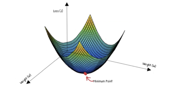
As we discussed in Module 4, the algorithm we use to navigate this landscape and find the minimum is gradient descent.

The Training Loop: The Four Key Steps

Training a neural network is an iterative process, often called the training loop. Each iteration involves four fundamental steps:

1. Forward Pass: Pass a batch of input data through the network to generate predictions.
2. Calculate Loss: Compare the network's predictions with the true target values using a loss function to get a single number representing the error.
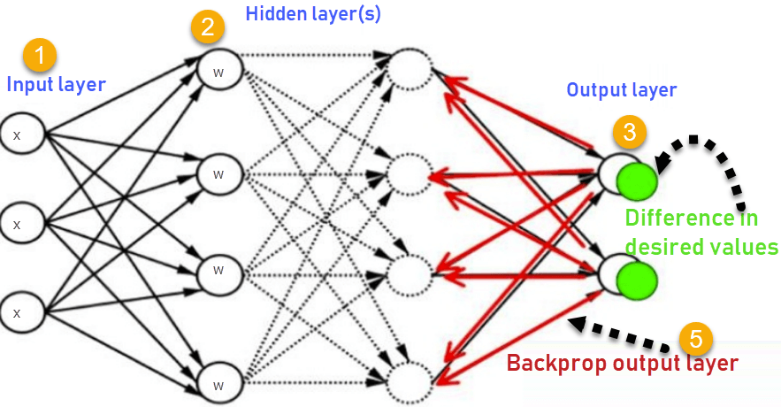
3. Backward Pass (Backpropagation): Calculate the gradient of the loss function with respect to every single weight and bias in the network. This tells us how much each parameter contributed to the overall error. This is the core new concept for today.
4. Update Parameters: Use the gradients calculated in the backward pass to update the weights and biases using the gradient descent update rule, taking a small step in the direction that most effectively reduces the loss.

This loop is repeated thousands or even millions of times, gradually adjusting the parameters until the network's predictions become accurate.

Backpropagation: The Engine of Learning

The most complex part of the training loop is the backward pass, which is powered by an algorithm called backpropagation. At its heart, backpropagation is simply a clever and highly efficient way to apply the chain rule from calculus to a complex, layered function like a neural network.

To understand this, it's helpful to visualize the network not just as layers, but as a massive computational graph, where every simple operation (addition, multiplication, activation function) is a node.

The following video provides an excellent, from-the-ground-up explanation of backpropagation. It starts with a simple curve-fitting problem and builds the concepts of a computational graph, the forward pass, and the backward pass. This will connect directly to your engineering background and your prior knowledge of derivatives.

To summarize the key ideas from the video:

• Forward Pass: Information flows from left to right through the computational graph. We start with inputs and parameters and compute all intermediate values until we arrive at the final loss.
• Backward Pass (Backpropagation): Information flows from right to left. We start with the gradient of the loss with respect to itself (which is just 1). Then, at each node, we use the chain rule to calculate the gradient of the loss with respect to that node's inputs, based on the gradient of the loss with respect to its output (which we already calculated from the node to its right).
• This process continues until we have the gradient of the loss with respect to the original parameters (the weights and biases), which is exactly what we need for gradient descent.

Now, let's see how this same idea applies specifically to the layers of a neural network.

The key insight here is that backpropagation is a process of credit assignment. It figures out exactly how "responsible" each weight and bias was for the final error and tells us how to nudge it to improve the result.

Gradient Descent: Putting the Gradients to Work

Once backpropagation has efficiently computed the gradient vector (the collection of all partial derivatives, $\frac{\partial L}{\partial w}$ and $\frac{\partial L}{\partial b}$), we perform Step 4 of our training loop: updating the parameters. This is done using the familiar gradient descent update rule:

${\theta }_{\text{new}}={\theta }_{\text{old}}-\alpha \nabla J(\theta )$

Where:

• $\theta$ represents a parameter (a weight or a bias).
• $\alpha$ is the learning rate.
• $\nabla J(\theta )$ is the gradient of the loss function $J$ with respect to the parameter $\theta$, calculated by backpropagation.

In practice, calculating the gradient over the entire dataset for every single update (Batch Gradient Descent) is too slow. Instead, we use more efficient variants.

Mini-batch Gradient Descent is the most common approach for training neural networks. It strikes a balance between the stability of using the full dataset and the speed of using a single example.

A Practical Example: Implementing the Training Loop

Let's walk through an article that puts all these concepts together into a Python implementation from scratch using NumPy. This will solidify your understanding of how the forward pass, backward pass, and parameter updates connect.

This implementation demonstrates that beneath the high-level abstractions of libraries like TensorFlow or PyTorch, the core logic is exactly what we've discussed: a loop that repeatedly performs forward propagation, calculates an error, uses backpropagation to find gradients, and applies gradient descent to update the parameters.

Conclusion

Congratulations! You have now connected all the fundamental components required to train a neural network. You've moved from understanding the static architecture to understanding the dynamic learning process.

Key Takeaways:

• Neural network training is an iterative training loop consisting of a forward pass, loss calculation, backward pass, and parameter update.
• Backpropagation is the algorithm used in the backward pass. It is an efficient application of the chain rule on the network's computational graph to calculate the gradient of the loss with respect to every parameter.
• Gradient Descent uses these calculated gradients to update the network's weights and biases, moving them in the direction that minimizes the loss.
• Mini-batch Gradient Descent is the standard, practical approach that balances computational efficiency and update stability.

Preview of the Next Lesson:

We now know how to train a network. But how do we know if the training is going well? A low loss on the training data doesn't always mean the model is good. In our next lesson, we will learn how to diagnose overfitting and underfitting by analyzing training and validation loss curves, a crucial skill for building models that generalize to new, unseen data.