Understanding Linear Regression: Minimizing the Sum of Squared Errors

What is Linear Regression?

At its heart, linear regression is about finding a linear relationship between variables. Imagine you have a dataset of houses, and you want to predict a house's price based on its size (in square feet). Linear regression attempts to do this by drawing a straight line through the data points that best represents the underlying trend.

This is called Simple Linear Regression because it involves only one predictor variable (size) and one target variable (price). The equation for this line is likely familiar to you:

$\hat{y}={\beta }_0+{\beta }_{1}x$

Where:

• $\hat{y}$ (y-hat) is the predicted price.
• $x$ is the size of the house.
• ${\beta }_1$ is the slope of the line. It tells us how much the price is predicted to change for a one-square-foot increase in size.
• ${\beta }_0$ is the y-intercept. It's the predicted price of a house with zero square feet (a theoretical baseline).

${\beta }_0$ and ${\beta }_1$ are the model parameters—the values we need to "learn" from the data.

But what if we have more information, like the number of bedrooms or the age of the house? We can extend the model to include multiple predictor variables. This is called Multiple Linear Regression. The equation simply expands:

$\hat{y}={\beta }_0+{\beta }_1{x}_1+{\beta }_2{x}_2+\cdots +{\beta }_p{x}_p$

Here, $x_1,x_2,\dots ,x_p$ represent the different features (size, bedrooms, age, etc.), and ${\beta }_1,{\beta }_2,\dots ,{\beta }_p$ are their corresponding coefficients.

For a clearer distinction between these two types, you can quickly review the following article.

Now, the main question is: how do we find the best values for ${\beta }_0$ and ${\beta }_1$? Out of all the infinite lines we could draw, which one is the "best fit"?

Finding the Best Line: The Concept of Error

To find the best line, we first need a way to measure how "bad" any given line is. We do this by calculating the error, or residual, for each data point. A residual is simply the vertical distance between an actual data point and the prediction made by our line.

• Actual value: $y_i$ (the true price of the i-th house)
• Predicted value: ${\hat{y}}_i$ (the price our line predicts for the i-th house)
• Residual for point i: $e_i=y_i-{\hat{y}}_i$

Let's watch a video that builds this intuition from the ground up.

The Sum of Squared Errors (SSE)

As the video explained, simply summing the residuals isn't useful because positive and negative errors cancel each other out. The standard solution is to square each residual before adding them up. This gives us a single, powerful metric for a model's total error: the Sum of Squared Errors (SSE), also known as the Residual Sum of Squares (RSS).

The formula for SSE is:

$\text{SSE}={\sum }_{i=1}^n(y_i-{\hat{y}}_i{)}^2$

This formula is the cornerstone of linear regression. It takes the error for each of the $n$ data points, squares it, and sums them all up.

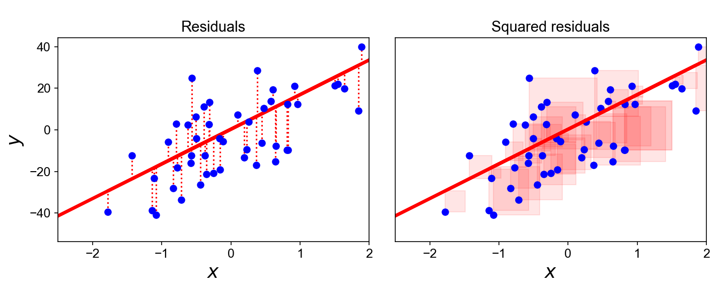
The Goal: Minimizing the Sum of Squared Errors

Now we have a way to score any potential line. A line with a high SSE is a poor fit, and a line with a low SSE is a good fit. The "best" line, therefore, is the one that results in the lowest possible SSE.

This transforms our task into an optimization problem, which should sound very familiar from our last module! We are trying to find the values of the parameters (${\beta }_0,{\beta }_1,\dots$) that minimize the SSE. This is why the method is called Ordinary Least Squares (OLS).

Let's continue the video to see this optimization concept in action.

Formulating the Optimization Problem

We can now formally state our goal. For simple linear regression, we substitute the line equation ${\hat{y}}_i={\beta }_0+{\beta }_1{x}_i$ into the SSE formula. This gives us the loss function we need to minimize:

$\underset{{\beta }_0,{\beta }_1}{\mathrm{minimize}}J({\beta }_0,{\beta }_1)={\sum }_{i=1}^n(y_i-({\beta }_0+{\beta }_1{x}_i){)}^2$

For multiple linear regression, the principle is identical, just with more parameters:

$\underset{{\beta }_0,\dots ,{\beta }_p}{\mathrm{minimize}}J({\beta }_0,\dots ,{\beta }_p)={\sum }_{i=1}^n(y_i-({\beta }_0+{\beta }_1{x}_{i1}+\cdots +{\beta }_p{x}_{ip}){)}^2$

This is the central formulation you need to understand. We have defined a loss function (SSE) that measures our model's error, and our goal is to find the parameters ($\beta$'s) that minimize this loss.

To see this formulation presented in a clear, textual format, please read the following brief section.

Why Use Squared Errors?

You might be wondering why we use the sum of squared errors and not, for instance, the sum of absolute errors. This is an excellent question, and it has deep connections to the optimization concepts you've learned.

Let's recap the two most important reasons:

1. Differentiability: The SSE function is a smooth, continuous curve (a parabola, in fact). This means we can calculate its gradient at any point. As you know from our work with gradient descent, being able to compute the gradient is essential for finding the minimum of a function. The absolute error function has a sharp corner at zero, where its derivative is undefined, making optimization much harder.
2. Penalizes Large Errors: By squaring the error, we penalize large mistakes much more heavily than small ones. An error of 10 contributes 100 to the SSE, while an error of 2 contributes only 4. This forces the model to pay more attention to avoiding significant outliers.

Conclusion

In this lesson, we established the fundamental principle of linear regression. We've moved from the abstract idea of a loss function to a concrete, powerful, and interpretable one.

Key Takeaways:

• Linear Regression models the relationship between variables by fitting a line (for simple regression) or a hyperplane (for multiple regression).
• The quality of the fit is measured by the residuals, which are the differences between the actual and predicted values.
• The overall model error is quantified by the Sum of Squared Errors (SSE), which is our loss function.
• The goal of linear regression is to find the model parameters ($\beta$'s) that minimize the SSE. This is known as the principle of Ordinary Least Squares (OLS).
• This formulation turns model fitting into an optimization problem, directly connecting to the methods we learned in the previous module.

Preview of the Next Lesson:

We now understand the objective of linear regression: to find the line that minimizes the sum of squared errors. In our next lesson, we will focus on the result. We'll learn how to interpret the coefficients ($\beta$'s), intercept, and the R-squared value of a fitted regression model to understand the relationships it has discovered in the data.