Hello! Welcome to your next lesson on Linear Regression.
In our last session, we focused on interpreting a fitted linear regression model. We learned what the intercept, coefficients, and R-squared value tell us about the relationship between our features and the target variable. This is crucial for understanding what the model has learned.
Today, we'll shift our focus to how the model's optimal parameters are found. We've previously touched upon Gradient Descent in our optimization module—an iterative process of taking small steps to find the minimum of a cost function. Now, we'll explore a more direct method specific to linear regression.
Our learning outcome for this lesson is to explain the purpose of the normal equations as a closed-form solution for least squares. We'll see how linear algebra provides an elegant and direct way to solve for the best-fit line, without any iterations at all.
From Iteration to a Direct Solution
To find the optimal parameters () that minimize the Sum of Squared Errors (SSE), Gradient Descent works by "walking" down the slope of the cost function. This is an iterative approach.
However, for linear regression, the cost function is a simple quadratic-like function (a convex paraboloid). For such functions, we can often find the minimum directly using calculus—by taking the derivative, setting it to zero, and solving. This direct, non-iterative method is called a closed-form solution. The Normal Equation is exactly this: an equation that gives us the optimal parameters in one single calculation.
To understand what a "closed-form" solution is, let's turn to an article that provides a clear definition and introduces the Normal Equation.
Normal Equation for Linear Regression Tutorial
The article 'Normal Equation for Linear Regression Tutorial' from DataCamp clearly explains the concept of a closed-form solution and introduces the Normal Equation in the context of linear regression's cost function.
Please read the first two sections, 'What is the Normal Equation?' and the section immediately following it that presents the formula. Focus on how it's described as an 'analytical approach' that directly minimizes the cost function.
As the article states, the Normal Equation is:
This might look intimidating, but it's just a compact way of expressing a solution using linear algebra. Let's break down how we get here.
Two Paths to the Same Equation
There are two powerful ways to understand where this equation comes from: a calculus-based derivation and a geometric one. Your engineering background gives you a great foundation for appreciating both.
1. The Calculus Approach: Finding the Bottom of the Bowl
The cost function for linear regression, , is the Sum of Squared Errors. In matrix form, it's written as:
Here:
- is the design matrix, with a row for each data sample and a column for each feature (plus an extra column of 1s for the intercept).
- is the vector of our model parameters (the intercept and all coefficients).
- is the vector of true target values.
- gives the vector of our model's predictions.
To find the minimum of this function, we calculate its derivative (gradient) with respect to and set it to zero. This is analogous to finding the bottom of a bowl where the slope is flat.
The video below provides a fantastic, step-by-step walkthrough of this derivation. It requires some comfort with matrix notation but explains each step clearly.
Linear Regression From Scratch in Python (Mathematical, Closed-Form)
The video 'Linear Regression From Scratch in Python' by NeuralNine derives the closed-form solution before implementing it. The derivation is clear and focused on the algebraic manipulation.
Watch the section from 07:45 to 18:44. Follow along as the presenter expands the Residual Sum of Squares (RSS) in matrix form, takes its partial derivative with respect to the parameters (beta), and sets it to zero to solve for the optimal parameters.
After all the algebraic steps, we arrive at the Normal Equation:
And solving for gives us our famous formula.
2. The Geometric Approach: The Power of Projections
This calculus derivation can feel a bit abstract. Fortunately, there's a more intuitive geometric interpretation that resonates well with vector concepts from engineering.
Imagine our target values y as a single vector in a high-dimensional space. The columns of our feature matrix X define a plane (or hyperplane) in that space, known as the column space. Any prediction our linear model can make, , must lie on this plane.
The goal of least squares is to find the prediction on the plane that is closest to our actual target vector y. Geometrically, the closest point is the orthogonal projection of y onto the plane.
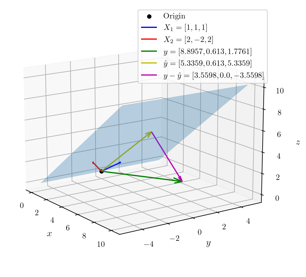
For the error vector to be orthogonal to the column space of , it must be orthogonal to every vector in that space. This is mathematically stated as:
Substituting , we get:
Distributing , we have:
And rearranging this gives us the Normal Equation once again:
This geometric view shows that the Normal Equation isn't just a result of calculus; it's a fundamental statement about finding the closest projection of a vector onto a subspace.
Test your understanding!
Imagine you have a single feature x and are trying to predict y. Your design matrix X has two columns: a column of 1s (for the intercept) and the column of x values. Why is the Normal Equation a system of two linear equations in this case? What do those two equations represent?
Show answer
In this case, is a 2-element vector [intercept, coefficient]. The matrix equation expands into a system of two linear equations with two unknowns ( and ).
These two equations correspond to setting the partial derivative of the cost function with respect to the intercept to zero, and the partial derivative with respect to the coefficient to zero. Solving this system gives you the values for the intercept and coefficient that simultaneously minimize the error.
Normal Equation vs. Gradient Descent: Which to Choose?
So we have two methods to find the optimal : the direct Normal Equation and the iterative Gradient Descent. Which one should you use? The choice depends almost entirely on the number of features in your dataset.
Let's read a clear comparison of the two approaches.
Normal Equation in Linear Regression
This article from GeeksForGeeks provides a direct comparison between the Normal Equation and Gradient Descent, highlighting their pros and cons.
Read the section 'The Normal Equation vs Gradient Descent'. Pay close attention to the trade-offs regarding computational complexity, the need for a learning rate, and feature scaling.
Here is a summary of the key differences:
| Feature | Normal Equation | Gradient Descent |
|---|---|---|
| Approach | Analytical, closed-form | Iterative |
| Learning Rate | Not required | Must be chosen carefully |
| Iterations | None | Many, until convergence |
| Feature Scaling | Not required | Required for good performance |
| Computational Cost | High, due to which is | Lower cost per iteration, scales better |
| Best for... | Datasets with a small number of features (n < 10,000) | Datasets with a very large number of features |
The bottleneck for the Normal Equation is calculating the inverse of . This is an matrix, where is the number of features. The complexity of matrix inversion is typically cubic, . This is fine for a few hundred or a few thousand features, but it becomes incredibly slow if you have, say, 100,000 features.
Gradient Descent, on the other hand, works well regardless of the number of features, making it the standard choice for the very large-scale problems common in modern machine learning.
Conclusion
In this lesson, we demystified the Normal Equation, seeing it as a powerful, direct method for solving linear regression. You now understand its purpose as a closed-form solution that analytically minimizes the least squares cost function.
Key Takeaways:
- The Normal Equation provides a direct, one-step solution to find the optimal parameters in linear regression, unlike the iterative Gradient Descent.
- The formula is derived by setting the gradient of the SSE cost function to zero.
- Geometrically, it represents finding the orthogonal projection of the target vector onto the space spanned by the features.
- The primary drawback is its computational complexity (), which makes it impractical for datasets with a very large number of features. For those cases, Gradient Descent is the preferred method.
Understanding both methods gives you a deeper appreciation for how models are trained and the trade-offs involved in different optimization strategies.
Preview of the Next Lesson:
Now that we have two powerful methods to fit our model, how do we know if a linear model was a good choice in the first place? Linear regression rests on several key assumptions (like linearity and constant variance of errors). In our next lesson, we will learn how to use residual plots to diagnose violations of these assumptions, a critical step in building robust and reliable models.