Scree Plots for Optimal Principal Components

1. What is a Scree Plot?

At its heart, a scree plot is a simple line plot or bar chart that shows the eigenvalues (or the percentage of variance explained) for each principal component, ordered from largest to smallest. The name comes from a geology term, "scree," which refers to the pile of broken rock fragments at the base of a cliff. The plot often resembles a cliff-face, with a steep drop-off followed by a flatter "rubble" area.

As the video illustrates, the scree plot helps us quickly visualize the importance of each component. The first few components (the "cliff") capture a large amount of variance, while the later components (the "scree") contribute much less.

Here is a typical example of what a scree plot looks like:

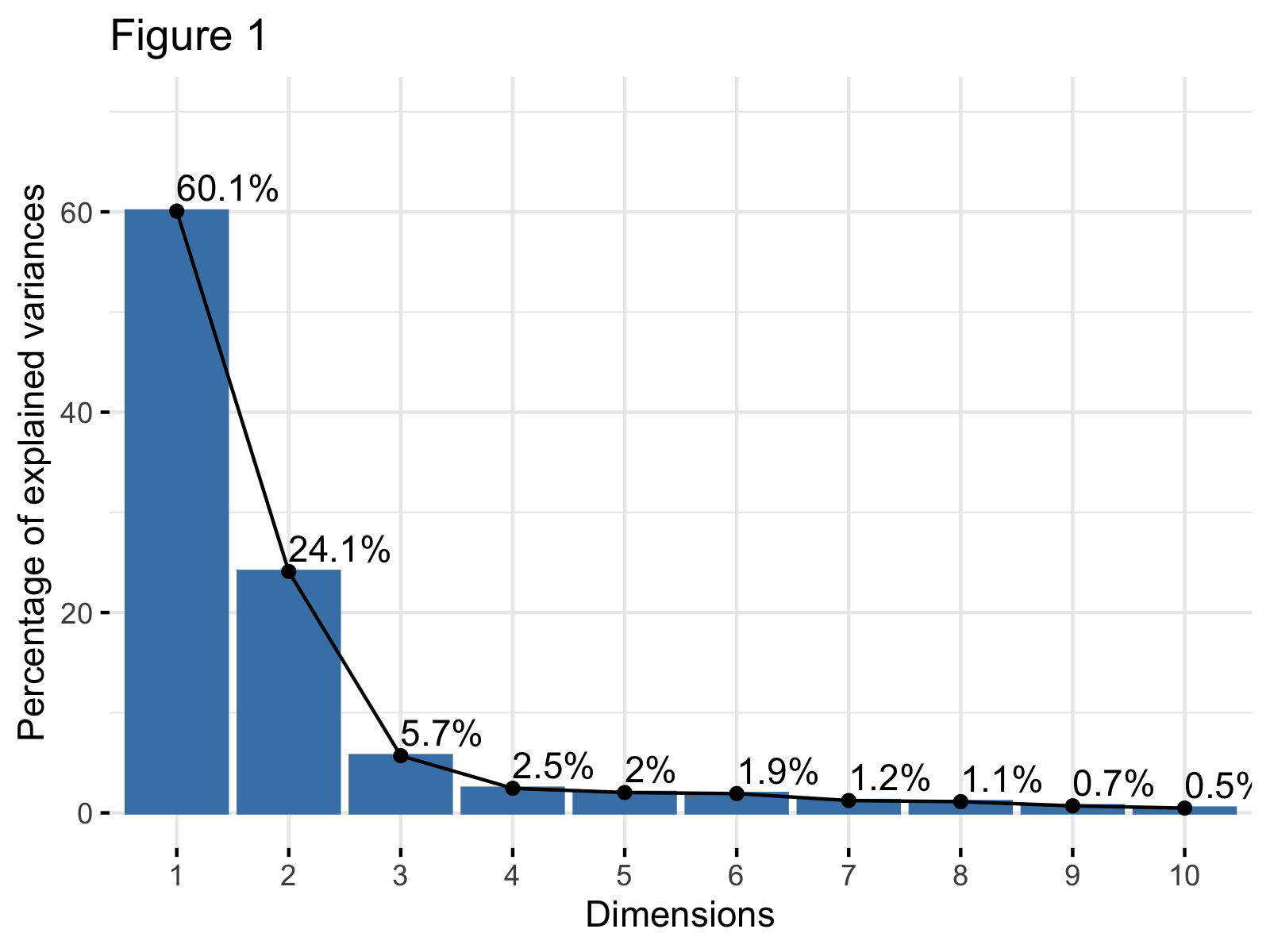
The y-axis shows the percentage of variance explained, and the x-axis lists the principal components. The goal is to find the "point of diminishing returns"—the point where adding another component doesn't give us much new information.

2. Methods for Selecting the Number of Components

Looking at a scree plot is one thing, but how do you formally decide on the number of components? There are several common heuristics, or rules of thumb, that can guide your decision. Let's explore three of the most popular ones.

Method 1: The Elbow Method

This is the most intuitive method and relates directly to the "cliff and scree" analogy. You look for the "elbow" in the plot—the point where the steep decline flattens out. The number of components at this elbow point is often considered the optimal number to retain. The components before the elbow are the ones that capture the most significant variance.

The main advantage of the elbow method is its simplicity. However, it can be subjective. Sometimes there is no clear elbow, or there might be multiple "elbows," making the choice less obvious.

Method 2: Cumulative Explained Variance Threshold

Instead of looking for an elbow, you can set a specific threshold for the total amount of variance you want to preserve. Common thresholds are 90%, 95%, or 99%.

To use this method, you plot the cumulative explained variance. This plot shows the percentage of total variance captured by the first k components. You then select the minimum number of components required to cross your desired threshold.

This method is less subjective than the elbow method because you set a clear, quantitative goal. The choice of threshold depends on your specific application. For data visualization, you might be happy with 80-90%. For input to a downstream machine learning model, you might want to retain 95% or even 99% to avoid losing potentially predictive information.

Method 3: Kaiser's Rule (Eigenvalue > 1)

Kaiser's rule provides a simple, objective criterion: keep only the principal components with an eigenvalue greater than 1.

The intuition behind this rule comes from working with standardized data. When you standardize your dataset before PCA (which is standard practice), each original variable has a variance of 1. Therefore, any principal component with an eigenvalue less than 1 is capturing less variance than a single original variable. The argument is that such a component is not contributing significant information and can be discarded.

This rule is easy to apply and removes all subjectivity. However, it is also considered by some statisticians to be too rigid and can sometimes lead to keeping too many or too few components compared to the other methods.

3. Practical Application in Python

Now let's see how these methods are applied in practice. The following video demonstrates how to generate a scree plot and use both the elbow method and Kaiser's rule to select the number of components for a real dataset using Python's scikit-learn library.

As the video shows, the process is quite straightforward:

1. Initialize and fit a PCA model on your scaled data, keeping all components for the initial analysis (n_components=None).
2. Extract the explained variance ratio (pca.explained_variance_ratio_) or the raw eigenvalues (pca.explained_variance_).
3. Plot these values to create your scree plot.
4. Apply your chosen heuristic (elbow, cumulative variance, or Kaiser's rule) to decide on the optimal number, k.
5. Finally, you would run PCA again, but this time setting n_components=k to get your final, transformed dataset.

Conclusion

In this lesson, you learned how to use one of the most important diagnostic tools for Principal Component Analysis: the scree plot. Making an informed decision about the number of components to keep is fundamental to using PCA effectively.

Key Takeaways:

• A scree plot visualizes the variance explained by each principal component, in descending order.
• The elbow method suggests choosing the number of components at the "bend" in the plot where the curve flattens.
• The cumulative variance threshold method involves choosing enough components to retain a desired percentage of the total variance (e.g., 95%).
• Kaiser's rule provides an objective guideline: keep components with an eigenvalue greater than 1.
• The choice is often a balance between simplicity (fewer components) and information retention (more components), and it's good practice to consider multiple heuristics.

Preview of the Next Lesson:

We have now concluded our deep dive into PCA, a powerful technique for dimensionality reduction. We will now shift our focus to another major pillar of unsupervised learning: clustering. In the next lesson, we will begin exploring how to find natural groupings in data by learning to apply the k-means algorithm to partition data into clusters.