Understanding Principal Components: Variance and Loadings

Hello! Welcome back to our module on Unsupervised Learning.

In our last lesson, we learned how to apply Principal Component Analysis (PCA) to reduce the dimensionality of a dataset. We walked through the process of standardizing data, finding the principal components, and transforming the data into a new, lower-dimensional space. However, applying PCA is only half the story. The real power comes from understanding what the results mean.

This lesson directly addresses our next learning outcome: Interpret principal components by examining the explained variance and component loadings. We will build on what we've learned to answer two critical questions:

How much information did we retain after reducing dimensions?
What do these new dimensions (the principal components) actually represent?

By the end of this 60-minute lesson, you will be able to confidently analyze the output of a PCA model, justify your choice of the number of components, and explain the meaning behind them—a key skill for moving from simply using ML tools to truly understanding them.

1. Explained Variance: How Much Information Do the Components Capture?

In the previous lesson, we established that PCA finds new axes (principal components) that maximize variance. The first principal component (PC1) captures the most variance, PC2 captures the second most, and so on. The amount of variance captured by each component is given by its corresponding eigenvalue.

A larger eigenvalue means that the component accounts for a larger proportion of the total variability in the data. This is the key to understanding how much information we are preserving.

Calculating the Proportion of Explained Variance

To make this practical, we don't usually work with the raw eigenvalue. Instead, we calculate the proportion of total variance that each component explains. For the i-th principal component, the calculation is straightforward:

Proportion of Variance Explained by PC_{i} = \frac{λ _{i}}{\sum _{j = 1}^{p} λ _{j}}

where $λ_{i}$ is the eigenvalue of the i-th component, and the denominator is the sum of all eigenvalues (which equals the total variance in the data).

This simple ratio tells you what percentage of the total information is captured by that single component.

Lesson 11: Principal Components Analysis (PCA)

For a formal definition and a clear explanation of this concept, let's look at a resource from Penn State's statistics program.

Please read the section titled 'How do we find the coefficients?'. Focus on the final two paragraphs, which start with 'Earlier in the course, we defined the total variation...'. This will show you exactly how the proportion of variance is calculated for a single component and for a set of components.

Cumulative Explained Variance

While knowing the variance of each component is useful, we are often more interested in the cumulative explained variance. This is the percentage of total variance captured by the first k components combined. We simply sum the proportions:

Cumulative Variance for first k PCs = i = 1 \sum k \frac{λ _{i}}{\sum _{j = 1}^{p} λ _{j}}

This cumulative value helps us decide how many components to keep. A common rule of thumb is to select enough components to explain a high percentage of the total variance, such as 95% or 99%. This creates a trade-off: fewer components mean a simpler model, but you might lose important information.

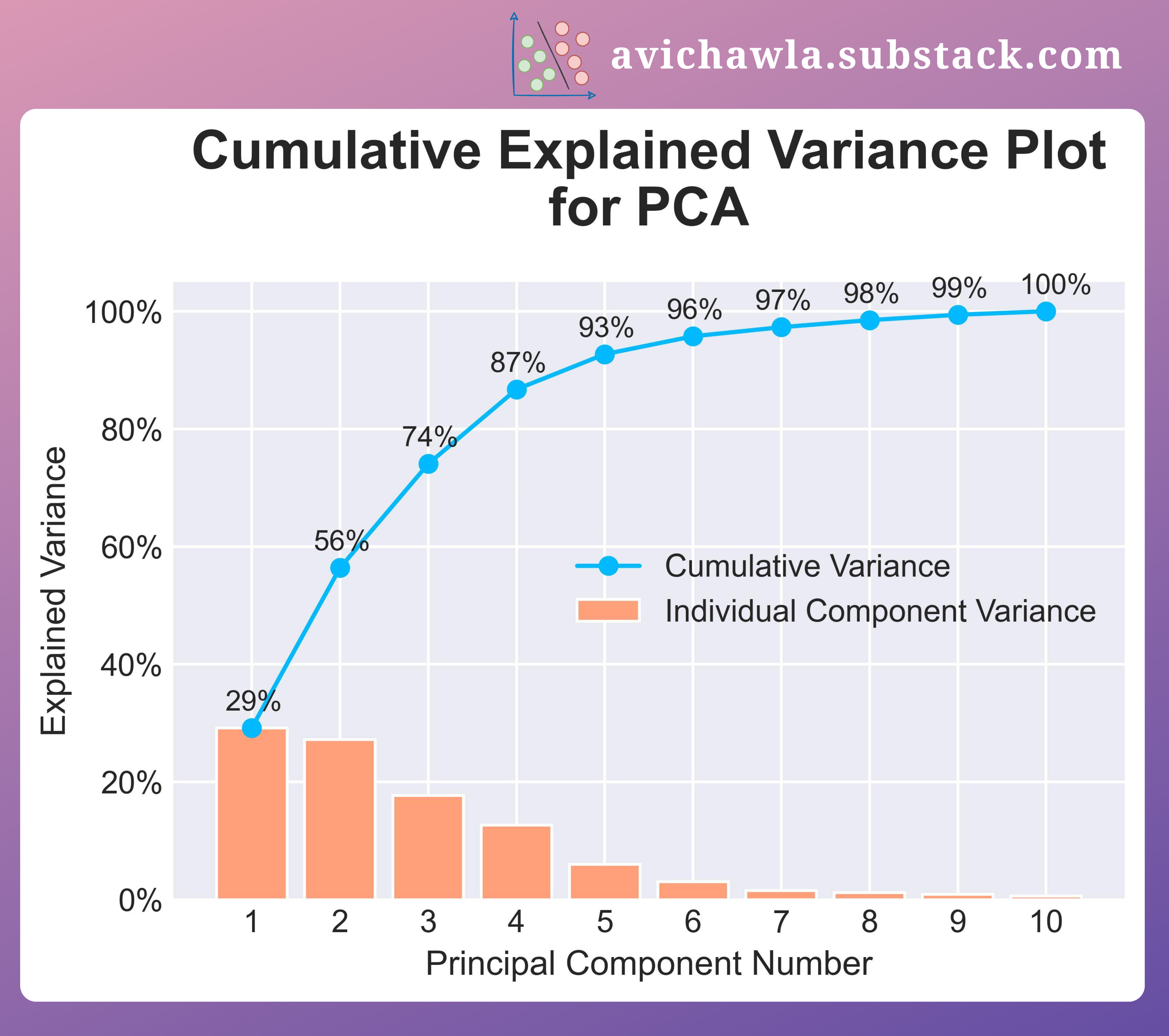
Cumulative Explained Variance Plot for PCA — This plot shows both the individual variance explained by each principal component (orange bars) and the cumulative variance (blue line). Notice how the first few components capture a large portion of the variance, while later components add progressively less information. We can see that the first 4 components capture 87% of the total variance.

In scikit-learn, you can access these values easily after fitting your PCA model.

# Assuming 'pca' is a fitted PCA object
explained_variance_ratio = pca.explained_variance_ratio_
cumulative_variance = explained_variance_ratio.cumsum()

print("Explained variance by each component:", explained_variance_ratio)
print("Cumulative explained variance:", cumulative_variance)

The explained_variance_ratio_ attribute gives you the proportion of variance for each component (our first formula). Using .cumsum() on this array gives you the cumulative explained variance.

2. Component Loadings: What Do the Components Mean?

Now that we know how to measure the information captured by our components, let's figure out what they mean. Remember, each principal component is a linear combination of the original features. For a dataset with features $X_{1}, X_{2}, \dots, X_{p}$ , the first principal component (PC1) can be written as:

PC_{1} = w_{11} X_{1} + w_{12} X_{2} + \dots + w_{1 p} X_{p}

The coefficients $w_{1 j}$ are called loadings. They are the elements of the eigenvector for that component. Loadings tell us how much each original feature $X_{j}$ contributes to that principal component.

Think of it like a recipe. The video you saw in the last lesson used a great analogy.

StatQuest: Principal Component Analysis (PCA), Step-by-Step

Let's revisit the 'StatQuest' video to refresh our memory on the 'cocktail recipe' analogy for interpreting principal components.

Please watch from 9:19 to 12:46. Pay close attention to how PC1 is described as a 'recipe' of Gene 1 and Gene 2. This section introduces the term 'loading scores' and explains that their relative size indicates the importance of each original variable to that component.

How to Interpret Loadings

To interpret a component, we look for the features with the largest loadings (in absolute terms, so large positive or large negative values are both important).

High positive loading: The feature contributes positively to the component. When this feature's value increases, the component's score tends to increase.
High negative loading: The feature contributes negatively. When this feature's value increases, the component's score tends to decrease.
Loading near zero: The feature has little to no influence on that component.

By examining the set of features with high loadings for a given component, we can often assign a meaningful, human-interpretable "name" to it. For example, if a component has high positive loadings for revenue, profit, and employees, we might call it a "Company Size" component.

Principal Component Analysis (PCA) - easy and practical explanation

The following video provides a practical explanation of how to use a 'loading plot' to visualize and interpret these relationships between original variables and principal components.

Watch from 4:13 to 6:40. This segment explains what principal component loadings are and how to interpret them from a plot. Notice how positively correlated variables cluster together, while negatively correlated ones appear on opposite sides.

In scikit-learn, the loadings are stored in the pca.components_ attribute. If you fit PCA on data with 10 features, pca.components_ will be an array where the first row contains the loadings for PC1, the second row contains the loadings for PC2, and so on.

Test your understanding!

You perform PCA on a dataset of car features and get the following loadings for PC1:

Feature	Loading on PC1
Horsepower	0.55
Engine Size	0.52
Weight	0.48
Miles Per Gallon (MPG)	-0.45

What does PC1 likely represent?

Show answer

PC1 likely represents a trade-off between power/size and fuel efficiency. High scores on PC1 correspond to cars that have high horsepower, large engines, and are heavy, but have low fuel efficiency (MPG). Low scores on PC1 would represent the opposite: smaller, more fuel-efficient cars.

3. Case Study: Interpreting PCA on Real Data

Let's tie these two concepts—explained variance and loadings—together with a practical example. We'll use the "Places Rated" dataset mentioned in the Penn State resource, which rates U.S. cities on nine criteria: climate, housing, health, crime, transportation, education, arts, recreation, and economy.

Lesson 11: Principal Components Analysis (PCA)

This article provides a fantastic, step-by-step interpretation of PCA results. It's a perfect example of how to turn the numbers from PCA into meaningful insights.

Please read section '11.4 - Interpretation of the Principal Components'. Focus on the table showing the correlations (which are equivalent to loadings for standardized data) and how the text below it interprets PC1, PC2, and PC3 by identifying the variables with the strongest correlations (e.g., correlations > 0.5).

Let's summarize the findings from that resource:

Look at the explained variance: The analysis (not shown in that specific section, but a standard first step) would reveal how much variance PC1, PC2, and PC3 capture. Let's assume they capture a significant amount, which is why we're interpreting them.
Interpret PC1: The resource notes that PC1 has strong positive correlations with Arts (0.985), Health (0.782), Transportation (0.585), Housing (0.544), and Recreation (0.520). It concludes that PC1 is a general measure of "urban quality and amenities." A city scoring high on PC1 would have good arts, health, and recreation facilities.
Interpret PC2: PC2 has a strong negative correlation with Health (-0.605). This component seems to isolate an aspect of "unhealthiness" or lack of healthcare quality that is separate from the general quality measured in PC1.
Interpret PC3: PC3 is strongly correlated with Crime (0.585) and Recreation (0.519). This is an interesting finding: it suggests a dimension where cities with higher crime also tend to have more recreation. This could be a real pattern (e.g., dense urban centers have both) or an artifact needing more investigation.

This process transforms abstract components into concrete concepts that help us understand the underlying structure of the data.

Conclusion

In this lesson, we moved beyond the mechanics of PCA to the art of interpretation. You learned how to use explained variance to quantify information loss and component loadings to understand the meaning of the principal components.

Key Takeaways:

Explained Variance tells you what percentage of the total information is captured by each principal component. The cumulative explained variance is used to decide how many components to retain to meet a desired threshold (e.g., 95%).
Component Loadings are the coefficients that define a principal component as a linear combination of the original features. They reveal which features are most important for each component.
By analyzing the loadings, you can assign an intuitive "name" or theme to each principal component, turning an abstract mathematical construct into a useful analytical tool.

Preview of the Next Lesson:

We've discussed using cumulative explained variance to choose the number of components. A very common visual tool for this decision is the scree plot. In the next lesson, we will focus specifically on how to use scree plots to select the optimal number of principal components, introducing a popular heuristic known as the "elbow method."

Recommended resources