Identifying Premium & Discount Zones Programmatically

1. The Core Concept: Premium, Discount, and Equilibrium

The fundamental principle of any business, including trading, is to buy assets cheaply and sell them at a higher price. In ICT, we formalize this with the concepts of Premium and Discount zones.

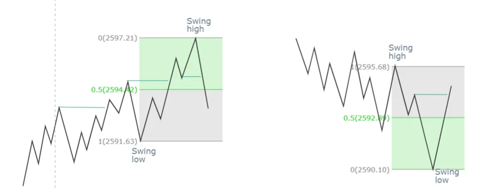
• Dealing Range: This is the price range between a significant swing low and a swing high.
• Equilibrium (EQ): This is the 50% level of the dealing range. It represents the "fair price."
• Premium: The area above the 50% equilibrium. Prices here are considered expensive. In a bearish market, this is where we look for optimal short-selling opportunities.
• Discount: The area below the 50% equilibrium. Prices here are considered cheap. In a bullish market, this is where we look for optimal buying opportunities.

These two images clearly illustrate the concept for both uptrends and downtrends.

To refresh your understanding of the logic and psychology behind these zones, the following video provides an excellent explanation.

2. Translating the Concept into Python Logic

Now, let's break down how to programmatically identify these zones. The logic follows three simple steps:

1. Define the Range: Identify the swing high and swing low that constitute your current dealing range. In a previous lesson (M6L1), you wrote a function to detect swing points. We will use that foundational work here.
2. Calculate Equilibrium: Find the midpoint of this range. The formula is simply:
   $\text{Equilibrium}=\frac{(\text{Swing High Price}+\text{Swing Low Price})}{2}$
3. Classify the Price: For any given candle, compare its closing price to the equilibrium level to determine if it's in a premium or discount zone.

This might sound simple, but applying it systematically is what gives it power. As this article about building an SMC-based trading bot highlights, this rule is a non-negotiable filter to prevent chasing price and improve trade quality.

3. Implementing Premium & Discount Zones in Code

We can implement this logic in Python. For this lesson, let's assume we have already identified a relevant swing low at $1.05 and a swing high at $1.10.

Our range is from $1.05 to $1.10.
Our Equilibrium would be: (1.10 + 1.05) / 2 = 1.075.

Any price above $1.075 is in premium, and any price below is in discount.

While we could write this logic from scratch, the smartmoneyconcepts Python library, which you've seen before, can help. It has a function specifically for this.

The smc.retracements function calculates how far the price has retraced into a range defined by swing points. A retracement of over 50% means the price has crossed the equilibrium.

Here is a complete script that:

1. Fetches price data.
2. Identifies swing highs and lows (using a function similar to what you built in M6L1).
3. Uses the most recent swing points to define a dealing range.
4. Calculates the premium/discount zones for the price action following that range.
5. Visualizes everything on a Plotly chart.

import pandas as pd
import yfinance as yf
import plotly.graph_objects as go
from smartmoneyconcepts import smc

# --- Step 1: Fetch Data ---
df = yf.download('EURUSD=X', start='2024-05-01', interval='4h')
df.reset_index(inplace=True) # Reset index to have 'Date' as a column for plotting

# --- Step 2: Identify Swing Highs and Lows ---
# Using the smc library for convenience, which functions like our previous work
df_swings = smc.swing_highs_lows(df, swing_length=15)

# --- Step 3: Define the Dealing Range ---
# Let's find the last major swing low and swing high to define our range.
# We'll work backwards from the most recent data.
last_swing_high = df_swings[df_swings['swing_high'] > 0].iloc[-1]
last_swing_low = df_swings[df_swings['swing_low'] > 0].iloc[-1]

# Determine which swing point is more recent to define the end of our range formation
if last_swing_high['Date'] > last_swing_low['Date']:
    range_high_price = last_swing_high['swing_high']
    range_low_price = df_swings[
        (df_swings['swing_low'] > 0) & 
        (df_swings['Date'] < last_swing_high['Date'])
    ].iloc[-1]['swing_low']
    range_start_index = df_swings[df_swings['swing_low'] == range_low_price].index[0]
    range_end_index = last_swing_high.name
    trend = 'bearish'
else:
    range_low_price = last_swing_low['swing_low']
    range_high_price = df_swings[
        (df_swings['swing_high'] > 0) & 
        (df_swings['Date'] < last_swing_low['Date'])
    ].iloc[-1]['swing_high']
    range_start_index = df_swings[df_swings['swing_high'] == range_high_price].index[0]
    range_end_index = last_swing_low.name
    trend = 'bullish'

print(f"Identified a {trend} range from {range_low_price:.5f} to {range_high_price:.5f}")

# --- Step 4: Calculate Equilibrium and Zones ---
equilibrium = (range_high_price + range_low_price) / 2.0

# --- Step 5: Visualize the Zones ---
fig = go.Figure(data=[go.Candlestick(x=df['Date'],
                                     open=df['Open'],
                                     high=df['High'],
                                     low=df['Low'],
                                     close=df['Close'],
                                     name='EURUSD')])

# Add the Premium Zone rectangle
fig.add_shape(
    type="rect",
    x0=df['Date'][range_start_index],
    y0=equilibrium,
    x1=df['Date'].iloc[-1], # Extend to the latest candle
    y1=range_high_price,
    line=dict(color="rgba(0,0,0,0)"),
    fillcolor="rgba(255, 0, 0, 0.2)", # Red for premium
    layer='below',
    name='Premium'
)

# Add the Discount Zone rectangle
fig.add_shape(
    type="rect",
    x0=df['Date'][range_start_index],
    y0=range_low_price,
    x1=df['Date'].iloc[-1], # Extend to the latest candle
    y1=equilibrium,
    line=dict(color="rgba(0,0,0,0)"),
    fillcolor="rgba(0, 255, 0, 0.2)", # Green for discount
    layer='below',
    name='Discount'
)

# Add a line for Equilibrium
fig.add_hline(
    y=equilibrium,
    line_dash="dot",
    annotation_text="Equilibrium (EQ)",
    annotation_position="bottom right"
)

fig.update_layout(
    title=f'EURUSD 4H with Premium & Discount Zones ({trend.capitalize()} Range)',
    xaxis_title='Date',
    yaxis_title='Price',
    xaxis_rangeslider_visible=False
)

fig.show()

When you run this code, it will generate an interactive chart. It will identify the last major price leg, calculate its 50% equilibrium level, and then shade the premium (red) and discount (green) zones for the entire area after the range was formed. This provides an immediate visual context for where the price is currently trading.

Conclusion

Congratulations on completing this module! You have now successfully automated the detection and visualization of several core ICT components: swing structures, fair value gaps, and now, premium/discount zones.

Key Takeaways:

• The market operates on the logic of buying low (discount) and selling high (premium).
• A dealing range (swing low to swing high) is the basis for our analysis.
• The equilibrium is the 50% level of this range and acts as a "fair value" line.
• The area below the equilibrium is the discount zone (ideal for buys in an uptrend), and the area above is the premium zone (ideal for sells in a downtrend).
• We can programmatically identify these zones by defining a range, calculating the midpoint, and then shading the areas on our chart.

Preview for the Next Lesson:
So far, our analysis has been focused purely on price action. But what about the dimension of time? The timing of price moves is just as critical as the levels they reach. In our next lesson, we will begin Module 7, "Time-Based Analysis and Price Cycles," by exploring the foundational ICT concept of the Power of 3 (Accumulation, Manipulation, and Distribution). This will open up a new layer of understanding in your market analysis.