Introduction
Welcome to the third module of your exam preparation course. In the previous module, we concluded our study of basic contingency table analysis by learning how to measure the strength of an association using relative risk and odds ratios. The odds ratio, in particular, will be a key concept moving forward.
Now, we shift from simply testing for and measuring an association to modeling it. This allows us to understand how one or more predictor variables relate to a response variable, enabling prediction and more complex inference.
The most common modeling tool you've likely encountered is Ordinary Linear Regression (OLR). However, as we'll see, it has significant limitations. This lesson focuses on a single, crucial objective: to explain the limitations of linear regression that motivate the need for a more powerful and flexible framework called Generalized Linear Models (GLMs). Understanding this "why" is the foundation for everything that follows.
The Assumptions of Ordinary Linear Regression
First, let's briefly recall the core assumptions of an ordinary linear regression model, often written as .
A standard linear model works well when its assumptions are met. These primarily are:
- Linearity: The relationship between the predictors (X) and the mean of the response (Y) is a straight line.
- Normality: The response variable Y, for any given value of X, is normally distributed. More precisely, the errors () are normally distributed.
- Constant Variance (Homoscedasticity): The variance of the response (and errors) is the same for all values of the predictors.
The image below provides a great visual summary of what these assumptions look like when they are met versus when they are violated.
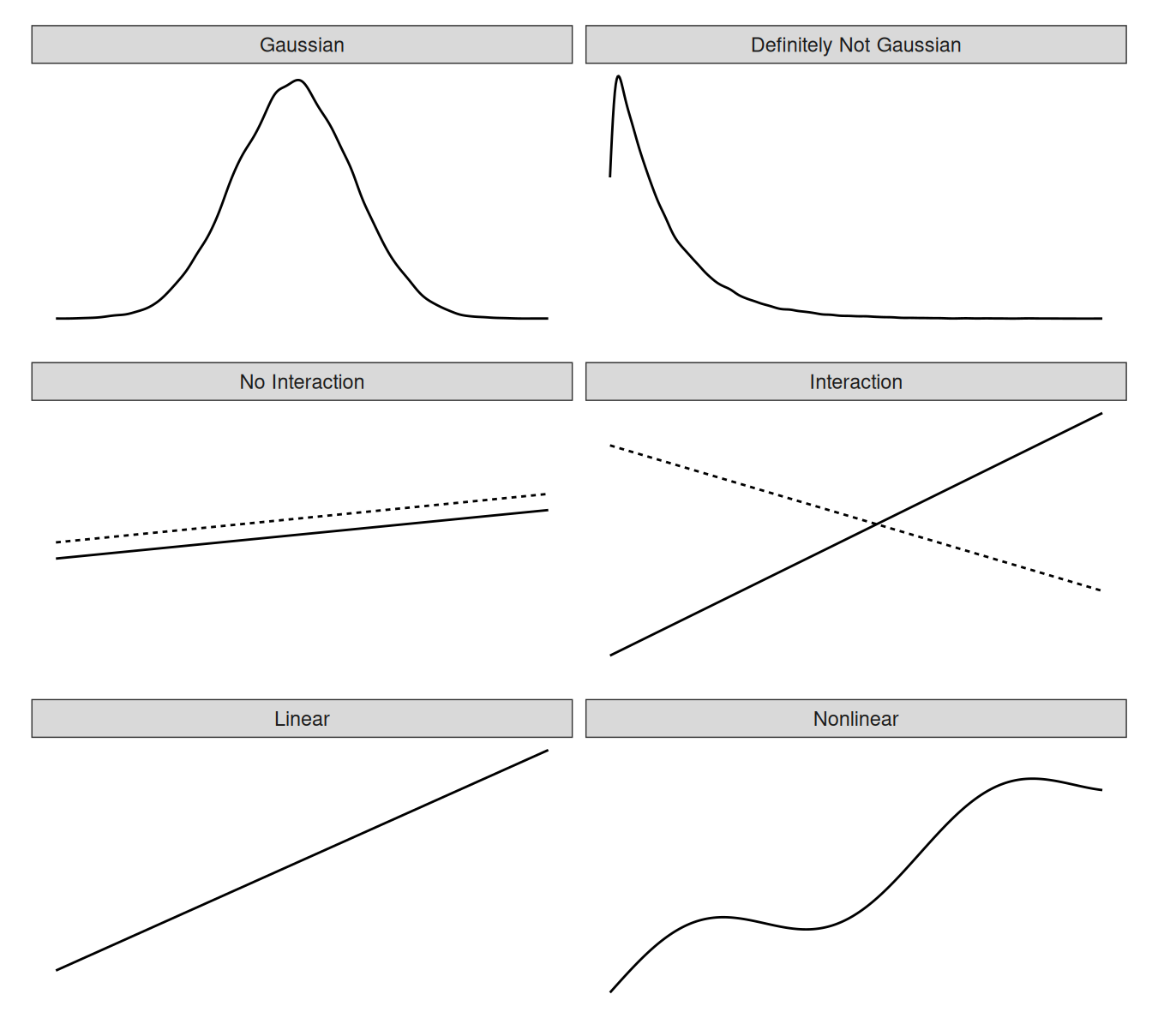
For your exam, much of the data you'll analyze—counts of events, binary outcomes like yes/no—will directly violate these assumptions. Let's explore exactly how.
When Linear Regression Fails
Applying linear regression to data that violates its core assumptions can lead to incorrect conclusions and nonsensical predictions. We'll look at two common data types you've already studied: binary outcomes and count data.
1. Binary Outcomes
Imagine you want to model whether a customer churns (Yes=1, No=0) based on their age. The response variable is binary, not continuous. This immediately creates several problems for linear regression.
To dig into the specifics, please read the section on "Binary Data" from the provided PDF resource. It clearly explains why a linear model is a poor choice in this scenario.
Generalized linear models for nonnormal response
This document from a statistics course at the University of South Carolina provides a detailed breakdown of why linear regression is inappropriate for binary data. It highlights issues with the mean, variance, and the physical meaning of predictions.
Please read the subsection titled 'BINARY DATA – THE BERNOULLI DISTRIBUTION' (starts on page 429). Focus on the three key problems identified: The response is only 0 or 1, which isn't a normal distribution. The variance depends on the mean, violating the constant variance assumption. A linear model can predict probabilities less than 0 or greater than 1, which is illogical.
Summary of problems with binary data:
- Non-Normality: The data follows a Bernoulli distribution (a single trial with two outcomes), not a Normal distribution.
- Non-Constant Variance: The variance is a function of the mean probability, , specifically . As the probability of the event changes, so does the variance.
- Nonsensical Predictions: The mean of a binary variable is the probability of the event occurring, which must be between 0 and 1. A linear regression line is unbounded and can easily predict values outside this range.
2. Count Data
Now consider modeling the number of support tickets a user submits in a week. This is count data—non-negative integers (0, 1, 2, ...). Linear regression also fails here, for similar reasons.
Watch this short video segment, which provides a concise explanation of the issues.
Regression with Count Data: Poisson and Negative Binomial
This video by Matthew E. Clapham clearly demonstrates the problems of applying linear regression to count data.
Watch from 00:34 to 01:26. The video points out three main issues when modeling counts with linear regression. Try to identify them before I list them below.
Summary of problems with count data:
- Non-Normality: Count data often follows a Poisson distribution, which is discrete and skewed, not a continuous and symmetric Normal distribution.
- Non-Constant Variance: For Poisson data, the variance is equal to the mean. As the average count increases, the variability around that average also increases. This violates the homoscedasticity assumption.
- Nonsensical Predictions: A linear model can predict negative counts, which is impossible in reality.
This last point is powerfully illustrated in the following image. Notice how the straight line of the linear regression model is a poor fit for the curving data and eventually dips into the negative territory, while the GLM (Poisson regression) provides a much more sensible fit.

Summary: Why We Need a More "General" Model
We've established that Ordinary Linear Regression is insufficient when its core assumptions are not met. The table below summarizes the key limitations we've discussed. This is a critical takeaway for your exam.
| Limitation of Linear Regression | Why It's a Problem for Categorical/Count Data | Example Data Type |
|---|---|---|
| Normality Assumption | The response is not bell-shaped (e.g., only two outcomes, or skewed counts). | Binary (Bernoulli), Count (Poisson) |
| Constant Variance Assumption | The variance changes with the mean (e.g., for binary, for Poisson). | Binary, Count |
| Unconstrained Range of Predictions | The model can predict impossible values (e.g., probabilities > 1, negative counts). | Binary, Count, Positive Continuous |
| Linearity Assumption | The relationship isn't a straight line (e.g., S-shaped for probabilities, exponential for counts). | Binary, Count |
This is precisely where Generalized Linear Models (GLMs) come in. They "generalize" the linear model to handle these exact situations. GLMs are not a single model, but a framework that allows you to:
- Model response variables from various distributions (not just Normal).
- Model variance that is not constant.
- Ensure predictions are sensible by using a link function to connect the predictors to the response.
To reinforce these ideas, I recommend reviewing the following practical guide.
Generalized Linear Models (GLM): When to Use Each Type
This practical guide from MCP Analytics provides a clear, application-focused summary of when to use GLMs. The FAQ section is particularly helpful for a quick review.
First, read the section 'When to Use This Technique' to see practical examples of where GLM is needed. Then, read the 'Frequently Asked Questions' at the end, specifically the first two questions that directly compare GLM and linear regression. This will help solidify the key decision rule for your exam.
Conclusion
In this lesson, we established the fundamental motivation for using Generalized Linear Models. You learned that Ordinary Linear Regression is built on a strict set of assumptions that are often violated by real-world data, especially the kinds of binary and count outcomes central to this course.
Key Takeaways:
- Ordinary Linear Regression assumes a Normal response distribution, constant variance, and a linear relationship.
- Binary and count data violate these assumptions, leading to problems like non-constant variance and the prediction of impossible values (e.g., probabilities > 1 or negative counts).
- GLMs were developed to overcome these limitations, providing a flexible framework for modeling diverse types of data.
You now understand why we need GLMs. In our next lesson, we will formally define the three core components of a GLM: the Random Component, the Systematic Component, and the Link Function. You'll see exactly how these parts work together to solve the problems we've identified today.