Reshaping Wide to Long Panel Data

1. Wide vs. Long Data: What and Why?

When you work with panel data—where you observe the same entities (like counties or children) at multiple points in time—the data can be structured in two primary ways.

• Wide Format: Each entity has a single row, and measurements from different time points are in separate columns. For example, you might have columns like placements_2020, placements_2021, and placements_2022.
• Long Format: Each row represents one observation of one entity at one point in time. You would have a column for the entity identifier (e.g., county_fips), a column for the time period (e.g., year), and a column for the value (e.g., placements).

For most analytical tasks in Python, the long format is strongly preferred. It's more flexible and works seamlessly with libraries like statsmodels for regression and seaborn for plotting. Imagine trying to plot a time trend of placements across 10 years in wide format; you'd be wrestling with 10 different columns. In long format, you can simply plot the placements column against the year column.

This structure also aligns with the concept of "tidy data," where each variable forms a column, each observation forms a row, and each type of observational unit forms a table.

2. Reshaping with pandas.melt()

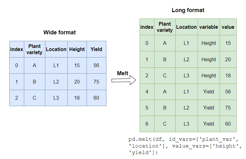
The primary tool for converting data from wide to long format in pandas is the .melt() function. It "unpivots" a DataFrame from a wide format to a long format.

Let's look at how it works.

Basic Melting

To see melt() in action, let's watch a quick tutorial.

As you saw, the basic syntax looks like this:

import pandas as pd




# Example wide-format DataFrame
df_wide = pd.DataFrame({
    'day': ['Monday', 'Tuesday', 'Wednesday'],
    'new_york': [32, 28, 30],
    'chicago': [25, 22, 27]
})

df_long = pd.melt(df_wide, 
                  id_vars=['day'], 
                  var_name='city', 
                  value_name='temperature')

print(df_long)

Output:

         day        city  temperature
0     Monday    new_york           32
1    Tuesday    new_york           28
2  Wednesday    new_york           30
3     Monday     chicago           25
4    Tuesday     chicago           22
5  Wednesday   chicago           27

Melting with Multiple Identifier Variables

In policy data, you often have multiple identifier variables, such as state_fips, county_fips, and year. You can pass a list of these columns to id_vars to keep them all fixed.

This is essential for your work, as you'll often need to preserve geographic identifiers alongside a time variable.

3. A More Complex Scenario: pandas.wide_to_long()

The melt() function is great, but it can be cumbersome when your wide-format data has multiple time-varying indicators. Consider a dataset from your previous lesson, where you merged AFCARS placement data with ACS poverty data. A wide version might look like this:

# A realistic wide-format child welfare dataset
data = {
    'county_fips': ['01001', '01003'],
    'county_name': ['Autauga County', 'Baldwin County'],
    'placements_2020': [50, 75],
    'poverty_rate_2020': [12.1, 15.3],
    'placements_2021': [55, 72],
    'poverty_rate_2021': [11.8, 15.5]
}
df_wide_complex = pd.DataFrame(data)

print(df_wide_complex)

Output:

  county_fips   county_name  placements_2020  poverty_rate_2020  placements_2021  poverty_rate_2021
0       01001  Autauga County               50               12.1               55               11.8
1       01003  Baldwin County               75               15.3               72               15.5

Here, we have two indicators (placements and poverty_rate) that both vary over time. While you could melt this, it would require multiple steps. A more direct tool is pandas.wide_to_long(). This function is designed for exactly this kind of structured naming convention (e.g., variable_year).

The key parameters for wide_to_long() are:

• df: The DataFrame to reshape.
• stubnames: A list of the "stubs" of the variable names (e.g., ['placements', 'poverty_rate']). pandas will look for columns that start with these stubs.
• i: The column(s) that identify the entities (similar to id_vars).
• j: The name for the new time-period column (e.g., year).
• sep: The character that separates the stub from the time value in the column name (e.g., _).

Here is how you would use it on our complex example:

# First, rename columns to have the year *before* the stub
# wide_to_long expects format like 'placements_2020', not '2020_placements'
# Let's adjust our thinking: often data comes as 'stubYEAR', e.g., 'placements2020'
# Let's recreate our dataframe to match the more common stub-first format
data = {
    'county_fips': ['01001', '01003'],
    'county_name': ['Autauga County', 'Baldwin County'],
    'placements_2020': [50, 75],
    'poverty_rate_2020': [12.1, 15.3],
    'placements_2021': [55, 72],
    'poverty_rate_2021': [11.8, 15.5]
}
df_wide_complex = pd.DataFrame(data)


df_long_complex = pd.wide_to_long(
    df_wide_complex,
    stubnames=['placements', 'poverty_rate'],
    i=['county_fips', 'county_name'],
    j='year',
    sep='_'
).reset_index()

print(df_long_complex)

Output:

  county_fips   county_name  year  placements  poverty_rate
0       01001  Autauga County  2020          50          12.1
1       01001  Autauga County  2021          55          11.8
2       01003  Baldwin County  2020          75          15.3
3       01003  Baldwin County  2021          72          15.5

As you can see, wide_to_long efficiently transformed the data, creating separate columns for each of the time-varying indicators, perfectly structured for longitudinal analysis.

The Payoff: What Long Format Enables

Now that your data is in long format, what can you do? This structure unlocks a powerful set of analytical techniques within pandas. For example, you can now easily use groupby() on your county identifiers to calculate changes over time or create lagged variables.

Conclusion

In this lesson, you've learned one of the most important data wrangling skills for longitudinal policy analysis. Transforming your data from wide to long format is the final, crucial step in preparing your data for modeling change over time.

Key Takeaways:

• Long format is the standard for longitudinal analysis in Python, making it easier to plot, model, and analyze data over time.
• pandas.melt() is the general-purpose tool for unpivoting data, ideal for simpler cases with one measured variable. You control it with id_vars, var_name, and value_name.
• pandas.wide_to_long() is a powerful, specialized tool for when you have multiple time-varying indicators with a consistent naming scheme (e.g., variable_year).

With your data now cleaned, merged, and properly shaped, you are ready to begin the analysis. In the next module, we will dive into Exploratory Analysis of Child Welfare Disparities. You'll start by using your long-format data to compute key child welfare indicators and generate summary statistics to identify patterns and disparities.