Addressing Missing Data in Child Welfare Records

1. The Challenge of Missing Data in Child Welfare Records

Missing data isn't just a technical nuisance; it's a reflection of real-world processes. In administrative datasets like AFCARS or NCANDS, data might be missing for many reasons: a field was optional, a record was expunged due to policy, a data system was updated, or there were simple data entry errors.

Handling this incorrectly can introduce significant bias. For example, if data on foster care placements is more likely to be missing from under-resourced rural counties, simply dropping those records could make your analysis systematically biased against the experiences of children in rural areas.

The paper highlights that dealing with missing data starts with understanding it. It's not just about finding NaN values; it's about identifying inconsistencies and making principled decisions on how to harmonize them, which can itself create missingness that must then be handled.

2. Identifying and Handling Missing Data with pandas

Let's turn to the practical side. We'll use the pandas library to find and handle missing data. The most common representation of a missing value is NumPy's np.nan (Not a Number).

This video provides an excellent, hands-on walkthrough of the essential pandas functions.

As you saw in the video, the first step is often a clean-up pass to ensure all missing or non-standard values are represented as np.nan. Here’s a summary of that workflow:

1. Load Data: When possible, use na_values in pd.read_csv() to automatically convert custom missing strings to np.nan.

   missing_formats = ['N/A', 'Not Reported', -99]
   df = pd.read_csv('your_data.csv', na_values=missing_formats)
   

2. Inspect: Use df.isna().sum() to get a count of missing values in each column.
3. Clean and Replace: For values not caught on import, use .replace() to standardize them, then cast the column to the appropriate data type.

   
   
   
   # Example inspired by the video and child welfare data
   # Let's say a 'placement_type' column has inconsistent codes
   # We decide to treat 'Unknown' and 'Other' as missing for our analysis
   df['placement_type'].replace(['Unknown', 'Other'], np.nan, inplace=True)
   
   
   
   
   # Example of numeric cleaning
   df['days_in_care'].replace('Less than a week', 3.5, inplace=True) # Approximate
   df['days_in_care'] = df['days_in_care'].astype(float) # Cast to float
   

3. Core Strategies: Deletion and Imputation

Once missing values are identified, you must decide what to do with them. The flowchart below shows a systematic way to think about the process.

The two simplest strategies are deleting the data or filling it with a single value.

Strategy 1: Deletion (Complete-Case Analysis)

This involves removing rows or columns that contain missing data.

• How: Use the df.dropna() method.
• When to Justify: This is only appropriate if the amount of missing data is very small and you can confidently assume the data is Missing Completely at Random (MCAR). MCAR means the fact that the data is missing has no relationship to any other data. For example, if a data entry form was smudged, causing a few random entries to be lost.
• The Risk: As the next video explains, this is rarely a safe assumption in social policy data. If missingness is systematic (e.g., related to geography, case complexity, or family income), dropping records will bias your sample and lead to incorrect conclusions.

Strategy 2: Single Imputation

This involves filling in missing values with a single, plausible value.

• How: Use the df.fillna() method.
• Common Choices:
  • Mean/Median: For numeric data. The median is generally preferred for skewed distributions, which are common in policy data (e.g., length of stay in foster care, income).
  • Mode: For categorical data (filling with the most frequent category).
  • Constant: Filling with a specific value like 0 or a string like "Unknown". This is useful when the missingness itself is meaningful.

Single imputation is better than listwise deletion because it preserves your sample size, but it should be used with caution. It can distort the statistical properties of your dataset by understating variability and weakening correlations.

4. An Advanced Strategy: Multiple Imputation

Simple imputation methods fail to account for the uncertainty associated with the missing values. We don't know the true value, so just picking one (like the mean) is a bit too certain. Multiple imputation addresses this.

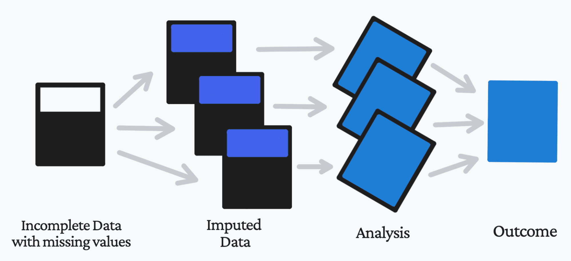
Multivariate Imputation by Chained Equations (MICE) is a popular and powerful multiple imputation method.

• The Idea: Instead of just using the column mean, MICE builds a regression model for each variable with missing data. It uses the other variables in the dataset as predictors to make an informed "guess" for the missing value.
• The Process: It iterates through the dataset, predicting and filling missing values for one variable at a time, and then repeats this process. This "chained" approach allows it to capture complex relationships and correlations in your data.
• The Benefit: By creating multiple imputed datasets, it allows you to see how sensitive your results are to the imputation and provides more accurate estimates of uncertainty (like standard errors in a regression model).

Here's how you might apply IterativeImputer in Python. Note that it's still considered an "experimental" feature in scikit-learn, so you need to explicitly enable it first.

import pandas as pd
import numpy as np




# Sample data with missing values
data = {'county_fips': ['01001', '01003', '01005', '01007'],
        'poverty_rate': [12.1, 15.3, np.nan, 25.0],
        'placement_rate': [5.2, np.nan, 8.9, 10.1]}
df = pd.DataFrame(data).set_index('county_fips')




# Import and enable the imputer
from sklearn.experimental import enable_iterative_imputer
from sklearn.impute import IterativeImputer




# Initialize the imputer
# It will create 5 different imputed datasets (n_nearest_features is not a MICE parameter, sample_posterior is)
# Let's use a simple version for demonstration
imputer = IterativeImputer(max_iter=10, random_state=0)




# Fit and transform the data
imputed_data = imputer.fit_transform(df)




# The output is a NumPy array, so convert it back to a DataFrame
df_imputed = pd.DataFrame(imputed_data, columns=df.columns, index=df.index)

print("Original Data:")
print(df)
print("\nImputed Data:")
print(df_imputed)

This approach is particularly powerful when you believe the data is Missing at Random (MAR), meaning the missingness can be explained by other observed variables in your dataset.

Conclusion

You now have a toolkit of strategies for handling missing data, from simple to advanced. Choosing the right one requires careful justification based on your data and your research goals.

Key Takeaways:

• Identification is Key: Missing data in administrative records is often hidden in non-standard formats. Your first step is always to explore and standardize these values to np.nan.
• Deletion is Risky: dropna() should only be used for small amounts of truly random missing data. In policy analysis, it's likely to introduce bias.
• Single Imputation is a Compromise: fillna() with the mean, median, or mode preserves your data but distorts its statistical properties. It can be a reasonable choice for exploratory analysis but is less ideal for final modeling.
• Multiple Imputation is Robust: MICE (via IterativeImputer) is a superior method for statistical modeling because it preserves relationships between variables and accounts for the uncertainty of imputation.
• Justification is Everything: There is no single "best" method. As a policy analyst, your report must include a section justifying your chosen strategy. You should explain why you believe the data is missing (e.g., MAR), what method you chose, and what its limitations are. As the child welfare paper (LINK) showed, sometimes the most honest approach is to acknowledge that certain data (like unsubstantiated reports) is systematically missing and limit the scope of your analysis accordingly.

In our next module, we will begin our Exploratory Analysis of Child Welfare Disparities. The first step will be computing key indicators from your now-cleaned, merged, and properly shaped data. The careful work you've done in this module to prepare the data is the essential foundation for all the analysis that follows.