Decision Trees: Construction, Splitting, and Pruning

The Intuition Behind Decision Trees

At its heart, a decision tree is an intuitive model that mimics human decision-making. Imagine trying to classify an email as spam or not. You might ask a series of questions: "Does the subject line contain the word 'winner'?", "Is the sender in my contact list?", "Does the email contain many capitalized words?". Based on the answers, you follow a path to a final decision. A decision tree formalizes this process.

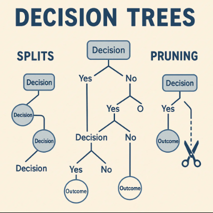
It's a flowchart-like structure where:

• Nodes represent a test on a feature (e.g., "petal width <= 0.8 cm?").
• Branches represent the outcome of the test (e.g., True/False).
• Leaf Nodes represent a class label (the final decision).

The algorithm learns this structure automatically from your training data through a process called recursive binary splitting.

The video below from StatQuest with Josh Starmer provides an excellent introduction to the terminology and structure of decision trees.

Building a Tree: The Splitting Process

The fundamental question in building a decision tree is: at each node, which feature and which split-point should we choose to divide the data? The goal is to select a split that makes the resulting child nodes as pure as possible. A pure node is one that contains data points from only a single class.

The algorithm uses a top-down, greedy approach. "Top-down" means it starts at the root node with the entire dataset and recursively splits it. "Greedy" means that at each step, it chooses the locally optimal split—the one that creates the purest child nodes at that moment—without looking ahead to see if a different split might lead to a better overall tree. Given your background in algorithms, you'll recognize this as a common heuristic for building complex structures efficiently.

To quantify "purity," we need a mathematical metric. The two most common metrics are Gini Impurity and Information Gain (which is based on Entropy).

Splitting Criterion 1: Gini Impurity

Gini Impurity is the default criterion in scikit-learn. It measures the probability of incorrectly classifying a randomly chosen element in the dataset if it were randomly labeled according to the class distribution in that node. The formula for a given node is:

where $C$ is the number of classes and $p_i$ is the probability of class $i$ in the node.

• A Gini Impurity of 0 means the node is perfectly pure (all samples belong to one class).
• A Gini Impurity of 0.5 (for a binary classification problem) indicates the highest level of impurity (samples are evenly split between the two classes).

The algorithm calculates the Gini Impurity for every possible split across every feature. It then chooses the split that results in the lowest weighted average Gini Impurity of the child nodes. The StatQuest video provides a brilliantly clear, step-by-step walkthrough of this entire calculation process for both categorical and numerical features.

Splitting Criterion 2: Entropy and Information Gain

An alternative to Gini Impurity is a concept from information theory: Entropy. Entropy measures the level of uncertainty or randomness in a node. The formula is:

Like Gini, an entropy of 0 signifies a perfectly pure node. The maximum value depends on the number of classes; for binary classification, it is 1.

The decision tree algorithm uses entropy to calculate Information Gain, which is the reduction in entropy achieved by splitting the data on a particular feature.

The algorithm aims to maximize the Information Gain, which is equivalent to minimizing the weighted average entropy of the children. The following article provides a detailed numerical example of this calculation.

While Gini Impurity and Information Gain are calculated differently, they generally produce very similar trees in practice. Gini is often preferred as the default because it's slightly faster to compute, as it avoids the logarithmic calculation.

Controlling Complexity: Overfitting and Pruning

If we allow a decision tree to grow until every leaf node is perfectly pure, it will likely overfit the training data. The tree will learn the noise and specific quirks of the training set, creating an overly complex model that fails to generalize to new, unseen data.

To combat this, we must control the tree's complexity using a process called pruning. There are two main approaches:

1. Pre-pruning (Early Stopping): This involves setting constraints on the tree's growth before training. We can define stopping conditions, such as:

   • max_depth: The maximum number of levels the tree can have.
   • min_samples_split: The minimum number of samples a node must have before it can be split.
   • min_samples_leaf: The minimum number of samples a leaf node must contain.
     If a split would violate any of these conditions, it is not performed.

2. Post-pruning: This involves growing the tree to its full depth and then trimming back branches that provide little explanatory power. The most common method is Cost Complexity Pruning (CCP). CCP introduces a tuning parameter, ccp_alpha, which acts as a penalty for the number of leaf nodes. As alpha increases, the algorithm is incentivized to prune away leaves, trading a small increase in training error for a simpler, more generalizable model.

The article we looked at earlier provides a good overview of these techniques.

Conclusion

In this lesson, we have dissected the inner workings of the decision tree algorithm. You've learned how these intuitive, flowchart-like models are constructed from data by making a series of greedy, locally optimal splits.

Key Takeaways:

• Decision trees are built using recursive binary splitting, a top-down, greedy process that aims to create the purest possible child nodes at each step.
• The "best" split is determined using a mathematical criterion to measure impurity. The two most common are Gini Impurity (probability of misclassification) and Information Gain (reduction in entropy).
• Unconstrained trees are highly prone to overfitting.
• Pruning is the essential technique to control tree complexity. This can be done through pre-pruning (setting hyperparameters like max_depth to stop growth early) or post-pruning (using methods like Cost Complexity Pruning to trim a fully grown tree).

In our next lesson, we will move from theory to practice. You will apply what you've learned to build, visualize, and evaluate a decision tree classifier in Python using scikit-learn. We will also discuss the primary strengths and weaknesses of this fundamental model, which will set the stage for understanding more advanced ensemble methods.