Hello! In our previous lesson, we delved into the theoretical underpinnings of decision trees, exploring how they are built through recursive splitting using criteria like Gini impurity and information gain. We also introduced the critical concepts of overfitting and pruning.
Today, we will build directly on that foundation to critically evaluate the decision tree algorithm. Our focus will be on answering the question: "When is a decision tree the right tool for the job?" To do this, we will systematically identify its primary strengths and weaknesses. You will learn why decision trees are celebrated for their interpretability but also why they must be handled with care due to their notorious tendency to overfit. Understanding these trade-offs is crucial before we move on to applying the algorithm in practice.
The Two Faces of a Decision Tree
A decision tree is a model of contrasts. It can be a simple, elegant, and highly interpretable tool, or it can become an overly complex, fragile model that fails to generalize. This duality is central to understanding the algorithm. Let's start by exploring its key advantages.
Strength: Unparalleled Interpretability
The most significant advantage of a decision tree is that it's a "white-box" model. This means its internal logic is transparent and easily understood. After training, you can visualize the entire model as a flowchart of if-then-else rules, which closely mimics human reasoning. This makes it incredibly valuable for explaining a model's predictions to non-technical stakeholders and for debugging the model's logic.
The following video from Emma Ding provides a concise overview of a decision tree's pros and cons. Pay close attention to her explanation of why interpretability is so powerful.
Decision Trees in Machine Learning: Easy Explanation for Data Science Interviews
This video, "Decision Trees in Machine Learning," discusses the practical advantages and disadvantages of the algorithm, which is a common topic in data science interviews.
Watch the segment discussing the first advantage, which focuses on how the tree structure allows us to easily understand feature importance and the logic behind predictions.
This transparency contrasts sharply with "black-box" models, such as neural networks, where even with a correct prediction, it can be very difficult to explain why the model arrived at that specific conclusion.
Other Key Strengths
Beyond interpretability, decision trees have several other practical advantages. The DataCamp tutorial, "Decision Tree Classification in Python," summarizes these nicely in a table.
Decision Tree Classification in Python Tutorial
This section of the tutorial provides a clear, tabulated summary of the pros and cons of decision trees.
Please read the section under the heading "Decision Tree Pros and Cons". As you read the "Advantages" column, focus on these two points in particular: Can easily capture non-linear patterns: Unlike linear models, which assume a linear relationship between features and the target, decision trees partition the feature space into rectangular regions, allowing them to model complex, non-linear relationships without feature transformations. Requires minimal data preprocessing: Decision trees are non-parametric, meaning they don't make assumptions about the statistical distribution of your data. Consequently, they are not sensitive to feature scaling (like standardization or normalization), which is a mandatory preprocessing step for many other algorithms like SVMs or Logistic Regression.
Weakness: The Tendency to Overfit
The single greatest weakness of a decision tree is its propensity to overfit the training data. As we discussed in the last lesson, if left unconstrained, the tree-building algorithm will greedily continue to split the data until every leaf node is perfectly pure. In doing so, it memorizes the training set, including any noise or outliers, creating an overly complex model that fails to generalize to new, unseen data.

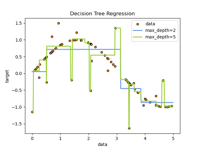
This phenomenon is not just for classification. The image below shows what happens in a regression context. The model with max_depth=5 (green line) twists and turns to hit every single data point, whereas the simpler max_depth=2 model (blue line) captures the general trend. The more complex model will perform poorly on new data points that don't follow the exact noisy pattern of the training set.
Emma Ding's video provides another excellent visual for how a single outlier can lead the tree to create convoluted decision boundaries.
Decision Trees in Machine Learning: Easy Explanation for Data Science Interviews
This segment of the video visually demonstrates how the presence of outliers can cause a decision tree to create unnecessarily complex splits.
Watch the section on the downsides of decision trees. Notice how the classification boundary on the right becomes distorted to account for the outlier points, a classic sign of overfitting.
How to See and Combat Overfitting
A key sign of overfitting is observing a high accuracy score on your training data but a significantly lower score on your test data. The GeeksforGeeks article "Overfitting in Decision Tree Models" provides a fantastic code-based demonstration of this. It trains multiple decision trees with increasing depth and plots their training versus testing accuracy.
Overfitting in Decision Tree Models
This article provides a focused, practical look at overfitting in decision trees and how to mitigate it using pruning.
Please read the entire section titled "Implementation of Pruning". You don't need to run the code yourself right now, but carefully follow the logic: Steps 1-6: Understand how the data is loaded and prepared. The key idea is creating depths = range(1, 20) to test trees of varying complexity. Step 7: This is the core of the demonstration. Notice how two models are trained in the loop: an overfit_model and a pruned_model (which is constrained by min_samples_leaf=4). For now, focus on the overfit_model. The code calculates and stores its score on both the training set (X_train) and the test set (X_test). Step 8: Look at the output plot. The Overfit Tree (Test) accuracy peaks and then starts to decrease as the tree depth increases. This is the classic signature of overfitting: adding more complexity (depth) beyond a certain point hurts performance on unseen data. The Pruned Tree (Test) accuracy is more stable.
This leads us to the other major weakness of decision trees.
Weakness: Instability and High Variance
Decision trees are highly sensitive to small variations in the training data. A minor change—even removing a few data points—can cause the greedy algorithm to select a different feature for an early split, leading to a cascade of changes and a completely different tree structure. This property is known as high variance.
This instability is a direct consequence of the hierarchical, greedy nature of the algorithm. Since the choice of each split depends on the preceding splits, small initial changes can have a large downstream effect.
The DataCamp article you reviewed earlier also lists this as a key disadvantage. This high variance can make the model feel unreliable.
From Weakness to Strength: A Preview of Ensembles
While the high variance and tendency to overfit are major problems for a single decision tree, these very weaknesses make it an excellent component for more advanced algorithms.
Ensemble methods, which we will cover soon, combine many "weak learners" to create one "strong learner." Decision trees are the quintessential weak learner. By training many different trees on slightly different subsets of the data (a technique called bagging) and averaging their predictions, we can dramatically reduce the variance and create a much more robust model. This is the core idea behind Random Forests. This directly addresses your interest in how algorithms evolve; Random Forest is a direct evolution designed to overcome the primary weaknesses of a single decision tree.
Conclusion
In this lesson, we have critically evaluated the decision tree algorithm, moving from the "how" of its construction to the "why" of its performance characteristics.
Key Takeaways:
- Strengths: Decision trees are highly interpretable ("white-box" models), can capture non-linear patterns, and require minimal data preprocessing like feature scaling.
- Weaknesses: Their primary drawbacks are a strong tendency to overfit the training data and high instability (variance), where small data changes can lead to vastly different models.
- The Central Trade-off: Controlling complexity via pruning (e.g., setting
max_depth) is a balancing act. A tree that is too simple will be biased and underfit, while a tree that is too complex will have high variance and overfit.
Now that you have a solid understanding of both the mechanics and the practical trade-offs of decision trees, you are ready to apply one. In our next lesson, we will get hands-on with scikit-learn to train, visualize, and evaluate a decision tree classifier on a real-world dataset.