Welcome back. In our previous lesson, we established a framework for deciding when to use an SVM, highlighting its strengths in high-dimensional spaces and its critical weakness: sensitivity to feature scaling. We concluded with the "golden rule" that you must always scale your features before training an SVM.
Today, we transition from theory to practice. This lesson is dedicated to applying what you've learned by building, training, and evaluating an SVM classifier using Python and scikit-learn. You will apply an SVM to a real-world dataset, experiment with different kernels to see how they impact the model's ability to find decision boundaries, and evaluate the resulting performance using metrics you are already familiar with. This hands-on experience is the final step in solidifying your understanding of this powerful algorithm.
The SVM Workflow: From Data to Prediction
The process of applying an SVM follows the standard machine learning workflow you've seen with other models, but with a special emphasis on the scaling step. We'll use the Breast Cancer Wisconsin dataset from scikit-learn, a classic binary classification problem, to walk through these steps.
The GeeksforGeeks article, "Classifying data using Support Vector Machines(SVMs) in Python," provides an excellent, self-contained walkthrough of this entire process. We will follow its structure closely.
Classifying data using Support Vector Machines(SVMs) in ...
This article provides a complete code implementation for an SVM classifier, from loading data to visualizing the result. We will use it as our guide.
Begin by reading through the sections "Implementing SVM Classification in Python" and "Visualizing the Decision Boundary". This will give you a complete overview of the steps involved. Pay close attention to Step 4: Scale the Features. Notice the use of StandardScaler. As we discussed, this is a non-negotiable step for SVMs. Recall from our earlier lessons on preprocessing why we use fit_transform on the training set but only transform on the test set. This prevents any information from the test set from "leaking" into the training process. Also, note that the example initially uses only two features (X = data.data[:,[0, 1]]). This is done to make the decision boundary easy to visualize in a 2D plot. In a real-world scenario, you would typically use all relevant features.
Experimenting with Kernels: The Key to Non-Linearity
The previous article focused on a linear kernel. While effective for data that is mostly linearly separable, the true power of SVMs comes from the kernel trick, which allows them to model complex, non-linear relationships. Let's explore how different kernels affect the model's performance.
As a reminder, the kernel function transforms our data into a higher-dimensional space where a linear separator can be found. This translates back to a non-linear boundary in the original feature space.

The most common kernels available in scikit-learn's SVC are:
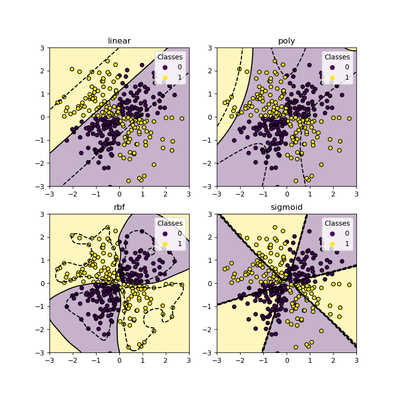
linear: A standard linear kernel. It's fast and a good baseline.poly: A polynomial kernel. It can model curved decision boundaries. Its complexity is controlled by thedegreehyperparameter.rbf(Radial Basis Function): The default and often most effective kernel. It can create highly complex, localized decision boundaries. Its behavior is controlled by thegammahyperparameter.sigmoid: This kernel function is similar to the activation function used in neural networks. It is less common in practice for SVMs but is available to try.
The image below shows how these different kernels produce vastly different decision boundaries on the same dataset.
Now, let's see this in action with code. The following article provides a very concise way to loop through different kernels and evaluate their accuracy.
How to implement SVM in Python - Replit
This resource demonstrates a simple loop to test multiple kernels.
Read the short code block in the section "Using different kernels with SVC". You can adapt this logic to the breast cancer dataset we've been using.
I encourage you to implement this yourself. Using the code from the GeeksforGeeks article as a base, create a loop that trains and evaluates an SVC for each of the four main kernels. Remember to use the scaled data for each one. You will likely observe that the rbf and linear kernels perform very well on this dataset, while poly and sigmoid might require more tuning to be competitive.
The Impact of Hyperparameters: C and gamma
Beyond just choosing a kernel, the performance of an SVM is critically dependent on its hyperparameters. As we've discussed, the two most important are:
-
C(Regularization Parameter): This parameter controls the trade-off between achieving a low training error and a low testing error.- A low
Cmakes the decision boundary smooth, prioritizing a larger margin. It allows more misclassifications of training points. - A high
Caims to classify all training examples correctly, potentially leading to a more complex decision boundary and overfitting.
- A low
-
gamma(Kernel Coefficient forrbf,poly,sigmoid): This parameter defines how far the influence of a single training example reaches.- A low
gammameans a single training example has a far-reaching influence, leading to a smoother, more general decision boundary. - A high
gammameans the influence is close, considering only points nearby. This can lead to a more complex, "wiggly" boundary that might overfit the training data.
- A low
The "codebasics" video provides a great hands-on demonstration of training an SVM and tweaking these parameters.
Machine Learning Tutorial Python - 10 Support Vector Machine (SVM)
This video walks through applying an SVM on the Iris dataset and shows the direct impact of changing hyperparameters.
Watch the segment where the model is trained and evaluated, from training the model. Notice the familiar train_test_split, SVC, .fit(), and .score() workflow. Next, watch the demonstration of parameter tuning. The presenter manually changes C, gamma, and kernel to see how the accuracy score changes. This is exactly the kind of experimentation you should be doing.
Try this on the breast cancer dataset. After you've found the best-performing kernel, experiment with different values for C (e.g., 0.1, 1, 10, 100) and, if you're using the rbf kernel, gamma (e.g., 0.01, 0.1, 1, 'auto', 'scale'). This manual tuning process gives you a strong intuition for how these parameters control the model's behavior.
While this manual approach is great for learning, it's inefficient for real projects. In a future lesson, we will cover automated hyperparameter tuning techniques like GridSearchCV, which systematically search for the optimal combination of parameters for you.
Conclusion
In this lesson, you have brought together all the theoretical components of Support Vector Machines and applied them to a practical problem. You have walked through the complete pipeline of loading, splitting, scaling, training, and evaluating an SVM classifier. Most importantly, you have experimented with different kernels and hyperparameters, gaining an intuition for how they influence the model's decision-making process and overall performance.
Key Takeaways:
- The practical workflow for SVMs is: Load -> Split -> Scale -> Train -> Evaluate. The scaling step is mandatory for good performance.
- The choice of kernel (
linear,rbf,poly, etc.) is a critical decision that determines the model's ability to handle non-linear data. - The hyperparameters
C(regularization) andgamma(kernel coefficient) control the bias-variance tradeoff, balancing between a smooth decision boundary (potential underfitting) and one that fits the training data very closely (potential overfitting). - Experimentation is key. Manually testing different kernels and tuning their parameters helps build a strong intuition for how SVMs work.
What's Next:
We have now concluded our in-depth look at supervised learning algorithms. You've covered everything from linear models to complex ensembles and SVMs. In the next module, we will pivot to Unsupervised Learning. We'll begin by exploring clustering, a set of techniques used to discover natural groupings in data when you don't have pre-defined labels. Our first algorithm will be one of the most famous and widely used: K-Means Clustering.