Understanding the Confusion Matrix

Why Accuracy Can Be Misleading

Imagine you've built a logistic regression model to detect a rare but critical disease. The model achieves 99% accuracy. On the surface, this sounds outstanding. But what if the disease only affects 1% of the population? A model that simply predicts "no disease" for everyone would also be 99% accurate, yet it would be completely useless—and dangerously so—as it would miss every single person who is actually sick.

This scenario highlights the core limitation of using a single accuracy score. It doesn't tell us what kind of errors our model is making. In many real-world applications, from medical diagnoses to fraud detection, the cost of one type of error is vastly different from another. We need a tool that gives us a more granular view.

The following article from Towards Data Science uses a cancer prediction example to illustrate this point perfectly.

As you've just read, misclassifying a sick patient as healthy (a False Negative) has far more severe consequences than misclassifying a healthy patient as sick (a False Positive). The confusion matrix is the tool that allows us to distinguish between these critical error types.

The Anatomy of a Confusion Matrix

A confusion matrix is a simple table that summarizes the results of a classification model by comparing the actual class labels to the predicted class labels. For a binary classification problem (e.g., "spam" vs. "not spam"), it's a 2x2 matrix.

The StatQuest channel provides one of the clearest and most intuitive explanations of the four components that make up this matrix.

To summarize and formalize the concepts from the video, let's define the four quadrants. Assume our goal is to identify a "positive" class (e.g., disease, spam, fraud) and a "negative" class (e.g., no disease, not spam, not fraud).

• True Positive (TP): The model correctly predicted the positive class.
  • Reality: Positive, Prediction: Positive.
• True Negative (TN): The model correctly predicted the negative class.
  • Reality: Negative, Prediction: Negative.
• False Positive (FP): The model incorrectly predicted the positive class. This is also known as a Type I Error.
  • Reality: Negative, Prediction: Positive.
• False Negative (FN): The model incorrectly predicted the negative class. This is also known as a Type II Error.
  • Reality: Positive, Prediction: Negative.

The following diagram provides a fantastic visual summary of this logic.

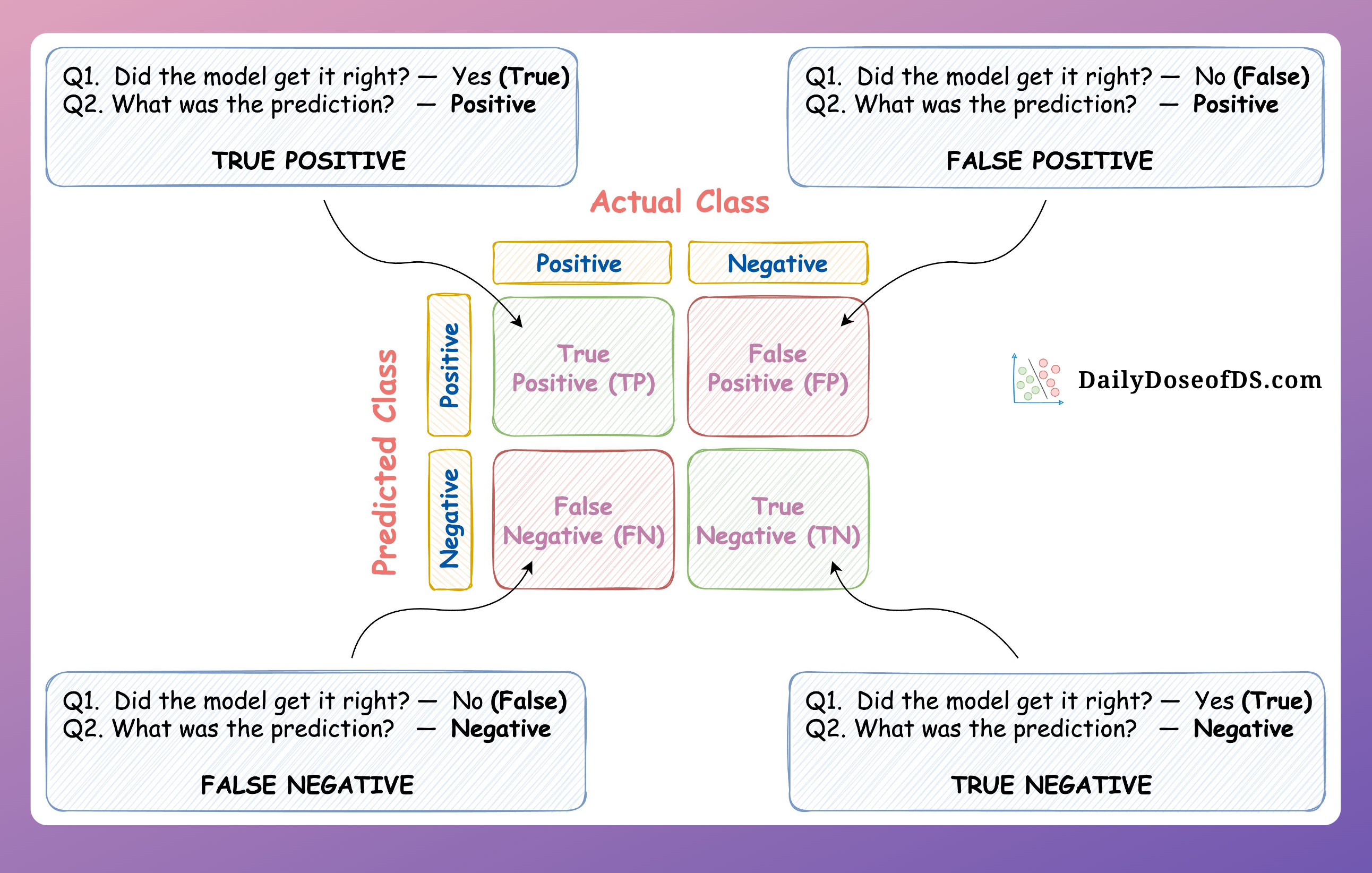
The diagonal elements (TP and TN) represent the correct predictions, while the off-diagonal elements (FP and FN) represent the errors. By looking at the distribution of values across these four cells, you can begin to understand your model's behavior.

Here is an example of a populated confusion matrix for a sickness prediction model.

Structuring and Interpreting the Matrix

The standard convention, used by Scikit-learn, is to place the Actual (True) Labels on the y-axis and the Predicted Labels on the x-axis.

Let's walk through another example to solidify this structure. The following reading from a DataCamp tutorial uses a spam detection scenario.

As you can see, constructing the matrix is a straightforward process of counting. The real value comes from interpreting what these counts mean for your specific problem.

• A high number of False Negatives (FN) might be unacceptable in medical screening, where failing to detect a disease is a critical failure.
• A high number of False Positives (FP) might be problematic in an email spam filter, where you risk sending important emails to the spam folder.

The Confusion Matrix in Practice with Python

Given your background, you'll appreciate seeing how this is implemented directly in code. Scikit-learn provides a simple function, sklearn.metrics.confusion_matrix, to do this for you.

The codebasics channel has a very practical walkthrough that connects the theory directly to the Python output.

Let's replicate that example to see it in action. Suppose we have the following true labels and predictions from a model classifying images as 'dog' (1) or 'not dog' (0).

import pandas as pd
import seaborn as sns
import matplotlib.pyplot as plt
from sklearn.metrics import confusion_matrix




# True labels
y_true = [1, 0, 1, 1, 1, 0, 0, 1, 0, 1] 



# Predicted labels from a model
y_pred = [1, 1, 1, 0, 0, 0, 1, 1, 0, 0]




# Generate the confusion matrix
cm = confusion_matrix(y_true, y_pred)

print("Confusion Matrix:")
print(cm)

Running this code produces the following output:

Confusion Matrix:
[[2 2]
 [3 3]]

Let's interpret this sklearn output, remembering that rows are y_true and columns are y_pred:

• cm[0, 0] = True Negatives (TN) = 2: The model correctly predicted 'not dog' 2 times.
• cm[0, 1] = False Positives (FP) = 2: The model incorrectly predicted 'dog' 2 times (when it was 'not dog').
• cm[1, 0] = False Negatives (FN) = 3: The model incorrectly predicted 'not dog' 3 times (when it was a 'dog').
• cm[1, 1] = True Positives (TP) = 3: The model correctly predicted 'dog' 3 times.

For better readability, it's common practice to visualize the matrix using a heatmap.

# Visualize the confusion matrix
plt.figure(figsize=(6, 5))
sns.heatmap(cm, annot=True, fmt='d', cmap='Blues', 
            xticklabels=['Not Dog', 'Dog'], 
            yticklabels=['Not Dog', 'Dog'])
plt.xlabel('Predicted Label')
plt.ylabel('True Label')
plt.title('Confusion Matrix for Dog Classifier')
plt.show()

This code will generate a clearly labeled and easy-to-interpret plot of your model's performance.

Conclusion

In this lesson, you've learned to look beyond simple accuracy and into the heart of a classification model's performance. The confusion matrix is an indispensable tool that provides a detailed account of a model's correct and incorrect predictions, breaking them down into four crucial components.

Key Takeaways:

• Accuracy alone can be a misleading metric, especially with imbalanced datasets or when the costs of errors are unequal.
• The confusion matrix is a table that summarizes a classifier's performance by comparing actual to predicted labels.
• Its four components are True Positives (TP), True Negatives (TN), False Positives (FP) (Type I error), and False Negatives (FN) (Type II error).
• The diagonal (TP, TN) represents correct predictions, while the off-diagonal (FP, FN) represents errors. Interpreting these errors is key to understanding model behavior.

You now have the foundational tool for classification evaluation. In our next lesson, we will build directly on this foundation to compute and interpret essential metrics derived from the confusion matrix: accuracy, precision, recall, and the F1-score. These metrics will allow you to quantify your model's performance in different ways, depending on the specific goals of your project.