Welcome to our next lesson on K-Nearest Neighbors. In our previous sessions, we established the theoretical foundation of KNN, exploring how it classifies data based on proximity and discussing its significant practical limitations, such as its sensitivity to feature scaling and the curse of dimensionality. Today, we bridge that theory with practice.
The goal of this lesson is to apply the KNN algorithm to a real-world classification problem using Python's scikit-learn library. You will learn the complete workflow: from preparing the data and building the model to, most importantly, tuning the hyperparameter 'K' for optimal performance and thoroughly evaluating the results. This practical application will solidify your understanding and demonstrate how the concepts we've discussed translate into code.
The Standard Workflow: From Data to Prediction
We will follow a structured, end-to-end process that is standard for many supervised learning tasks. This involves loading and preparing the data, splitting it for training and validation, applying necessary preprocessing (like scaling), training the model, and finally, evaluating its performance.
For this practical exercise, we will use a Kaggle notebook that provides a clear, step-by-step implementation. It uses a dataset where the goal is to predict whether a user will purchase a product based on their age and estimated salary.
kNN Classifier Tutorial - Kaggle
This Kaggle notebook by Prashant Banerjee will serve as our guide. It walks through a complete KNN implementation, from data loading to model evaluation. We will focus on the core coding steps.
Please follow along with the code in the notebook. Familiarize yourself with the initial data exploration in sections 7 and 8, but focus your main attention on the implementation steps that follow. Begin with Section 10: Split data into separate training and test set. Read the code and short explanation for splitting the data. This step is crucial to prevent data leakage. Next, study Section 12: Feature Scaling. Read the code where the StandardScaler is applied to the data. As we discussed, this is a mandatory step for distance-based algorithms like KNN. Finally, look at Sections 13-15. Review the code for instantiating and fitting the KNeighborsClassifier and for making predictions. Note the use of n_neighbors=5, which is the default 'K' value we are starting with.
Understanding the Role of 'K': The Bias-Variance Tradeoff
Before we tune 'K', it's essential to understand why we're tuning it. The choice of 'K' directly controls the model's complexity and embodies the classic bias-variance tradeoff.
- A very small 'K' (e.g., K=1) results in a model with low bias and high variance. The decision boundary will be highly flexible and can closely follow the training data, making it very sensitive to noise and individual data points. This often leads to overfitting.
- A very large 'K' results in a model with high bias and low variance. The decision boundary will be very smooth and may ignore local patterns in the data. The model is simpler and more generalized but may fail to capture the true underlying relationship, leading to underfitting.
The image below perfectly illustrates this. On the left, with K=1, the decision boundary is jagged and complex, trying to perfectly classify every single point. On theright, with K=100, the boundary is much smoother, averaging over a large neighborhood and ignoring the finer details.
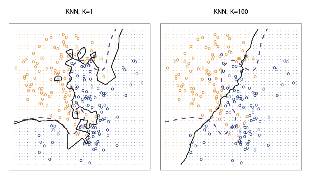
Our goal is to find a 'K' value that strikes a balance, creating a model that generalizes well to new, unseen data.
Method 1: Finding the Optimal 'K' with the Elbow Method
The most intuitive way to find the best 'K' is to iterate through a range of values, train a model for each, and plot their performance. We are looking for the "elbow point" in the graph—the point of diminishing returns where increasing 'K' no longer significantly improves the model's performance on the validation set.
This method provides a powerful visual inspection of how the model behaves at different complexity levels. The following article demonstrates this technique clearly.
Choosing the Right Number of Neighbors (k) for the K- ...
This article from Towards Data Science details several methods for choosing 'K'. We will focus on the first method, which uses visualization and cross-validation.
Please read Method 1: Visualizing classification performance on different k values (visual inspection). Pay close attention to the Python code, which loops from K=1 to 30. Notice that it uses cross_val_score to get a more robust estimate of accuracy for each 'K', a technique you're already familiar with. The resulting plot clearly shows how accuracy changes as 'K' increases, allowing you to identify the optimal "elbow" range.
This visual approach is often sufficient and provides great insight. The plot you generate will typically show high accuracy at low 'K' values (reflecting overfitting on the training data) and then stabilize or decrease as 'K' gets too large (underfitting).
Method 2: Automated Tuning with GridSearchCV
While the elbow plot is intuitive, scikit-learn provides a more automated and rigorous tool called GridSearchCV. This function performs an exhaustive search over a specified parameter grid (in our case, a list of 'K' values) and uses cross-validation to determine the hyperparameter that yields the best performance.
This automates the loop we saw in the elbow method and is a standard practice for hyperparameter tuning in machine learning workflows.

The same article we just reviewed also provides a concise example of using GridSearchCV.
Choosing the Right Number of Neighbors (k) for the K- ...
This section demonstrates the more automated GridSearchCV approach.
Please read Method 2: Finding the best k value using Grid Search hyperparameter optimization. The code is more compact because GridSearchCV handles the looping and cross-validation internally. After fitting, you can directly access the best parameter (gs.best_params_) and the corresponding score (gs.best_score_).
Evaluating the Final Model
Once you have determined the optimal 'K', you can train your final model using that value on the entire training set. The final step is to evaluate its performance on the held-out test set, which the model has never seen before.
The codebasics video below offers a great walkthrough of the evaluation process, including interpreting the confusion matrix and classification report.
Machine Learning Tutorial Python - 18: K nearest neighbors classification with python code
This video provides a practical demonstration of training a KNN model and, importantly, evaluating its performance with standard scikit-learn tools.
Watch the segment from this point. The presenter demonstrates how to: Calculate the accuracy score. Generate and interpret a confusion matrix, explaining what the diagonal and off-diagonal elements represent. Use a classification report to see precision, recall, and F1-score for each class.
For Deeper Insight: Building KNN From Scratch
Given your strong background in computer science and algorithms, you might find it insightful to see how KNN can be implemented from scratch. This exercise peels back the scikit-learn abstraction and forces you to think about the core mechanics: calculating Euclidean distance, iterating through data points, and finding the majority class.
The following video provides an excellent, concise tutorial on building a KNN classifier in Python using only NumPy.
How to implement KNN from scratch with Python
This video from AssemblyAI walks through a from-scratch implementation of the KNN algorithm, which will connect directly with your knowledge of data structures and algorithms.
Watch the two main segments of the video: Implementation: Pay attention to how the class is structured with fit and predict methods, how Euclidean distance is calculated, and how numpy.argsort is cleverly used to find the nearest neighbors. Application: See how the custom-built classifier is applied to the Iris dataset and its accuracy is calculated, proving the implementation works.
This is an optional but highly recommended step to deepen your algorithmic understanding of KNN.
Conclusion
In this lesson, you have moved from KNN theory to hands-on application. You have learned the complete practical workflow in scikit-learn and, most critically, how to tune the 'K' hyperparameter.
Key Takeaways:
- The standard machine learning workflow includes a train-test split followed by feature scaling, especially for distance-based models like KNN.
- The choice of 'K' is a classic example of the bias-variance tradeoff. Small 'K' leads to high variance (overfitting), while large 'K' leads to high bias (underfitting).
- The "elbow method" is an intuitive visual technique to find a good 'K' by plotting accuracy against different 'K' values.
GridSearchCVprovides a more robust and automated way to perform hyperparameter tuning using cross-validation.- A thorough model evaluation involves not just accuracy but also tools like the confusion matrix and classification report to understand performance on a per-class basis.
In our next lesson, we will shift gears and explore a completely different type of classifier: Naive Bayes. Unlike the geometric, distance-based approach of KNN, Naive Bayes is a probabilistic model rooted in Bayes' theorem, offering a new perspective on classification.