Assumptions of Linear Regression

Why Do Assumptions Matter?

Applying a linear regression model without checking its assumptions is like using a powerful tool without reading the safety manual—you might get a result, but it could be dangerously wrong.

To see a classic illustration of this, please watch this short introductory video. It uses a famous dataset called "Anscombe's Quartet" to show four very different datasets that produce the exact same statistical results, proving that you can't just trust the numbers blindly.

As the video shows, checking assumptions helps ensure that our model is a valid and reliable representation of the underlying relationships in our data.

The Key Assumptions of Linear Regression

There are several key assumptions that a linear regression model relies on. This image provides a great visual overview of what it looks like when these assumptions are met versus when they are violated. We will explore each of these in detail.

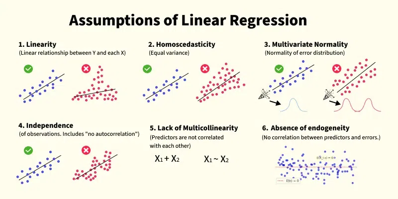
The main assumptions we will cover are:

1. Linearity
2. Homoscedasticity (Constant Variance of Errors)
3. Normality of Errors
4. Independence of Errors (No Autocorrelation)
5. No Multicollinearity

For each assumption, we will discuss what it means, why it's important, and how you can spot violations. The following in-depth video will be our guide.

1. Linearity

• What it is: The Linearity assumption states that the relationship between the predictor variables (X) and the target variable (Y) is linear. Essentially, the model assumes that a straight line is the best way to describe the relationship.
• Why it matters: If the true relationship is curved (non-linear), forcing a straight line through it will result in a model that makes systematic errors. Both the model's coefficients and its standard errors will be unreliable, rendering the entire model output useless.
• How to check: The most common way is to examine a residual plot, which graphs the model's errors (residuals) against the predicted values. If the assumption is met, you should see a random scatter of points around the zero line. If you see a U-shape, an inverted U-shape, or any other clear pattern, the linearity assumption is likely violated.

To explore this concept further, watch this segment from the video "Regression assumptions explained!".

2. Homoscedasticity (Constant Error Variance)

• What it is: This term, while complex-sounding, means "same variance." The assumption is that the errors (residuals) of the model have a constant variance across all levels of the predictor variables.
• Why it matters: When this assumption is violated (a condition called heteroscedasticity), the standard errors of the coefficients become unreliable. This directly impacts your p-values and confidence intervals. You might incorrectly conclude that a variable is not significant when it actually is, or vice-versa. The coefficients themselves remain unbiased, but our ability to test their significance is compromised.
• How to check: Again, we use a residual plot. Homoscedasticity is indicated by a random cloud of points with a consistent vertical spread. Heteroscedasticity often appears as a cone or fan shape, where the spread of the residuals increases or decreases as the predicted values change.

This next video segment explains this concept with a great example about income and expenditure.

3. Normality of Errors

• What it is: This assumption states that the model's errors (residuals) are normally distributed, with a mean of zero.
• Why it matters: The normality assumption is important for conducting valid hypothesis tests on the coefficients (i.e., for the p-values to be reliable). However, this assumption is considered "weaker" than others, especially with large sample sizes. Due to the Central Limit Theorem, the distribution of the coefficients tends towards normal even if the errors aren't, provided you have enough data.
• How to check: You can check this by creating a histogram or a Q-Q (Quantile-Quantile) plot of the residuals. A histogram should look roughly like a bell curve centered at zero. In a Q-Q plot, the points should fall closely along a straight diagonal line.

Within Alteryx, the Linear Regression tool's report output provides a histogram of the residuals, making this check straightforward.

Now, let's watch the video explanation for a deeper dive.

4. Independence of Errors (No Autocorrelation)

• What it is: This assumption requires that the errors are independent of one another. In other words, the error for one observation should not provide any information about the error for another observation.
• Why it matters: A violation, known as autocorrelation or serial correlation, is most common in time series data, where an event at one point in time can influence subsequent points. Like heteroscedasticity, autocorrelation makes your standard errors unreliable, leading to incorrect conclusions about the significance of your predictors.
• How to check: This is often checked by plotting the residuals against the order of the data (e.g., time). If there is a pattern (like a snaking or wave-like shape), the assumption is violated. Statistical tests like the Durbin-Watson test are also used.

The next video segment explains this with a stock index example.

5. No Multicollinearity

• What it is: This assumption applies to multiple linear regression (models with more than one predictor). It states that the predictor variables should not be highly correlated with each other.
• Why it matters: If two predictors are highly correlated, the model has trouble distinguishing their individual effects on the target variable. This leads to unreliable and unstable coefficient estimates. You might see a coefficient's sign flip unexpectedly or have very large standard errors, making the predictors appear insignificant even when they are important.
• How to check: You can check for multicollinearity by creating a correlation matrix between all predictor variables. A more formal method is to calculate the Variance Inflation Factor (VIF) for each predictor. A common rule of thumb is that a VIF value greater than 5 or 10 indicates a problematic level of multicollinearity.

The final video segment explains this tricky concept.

For a comprehensive textual reference on all these assumptions, including details on statistical tests and remedial measures, the article "Linear Regression Assumptions – Why is it important" from Towards Data Science is an excellent resource.

Conclusion

You've done an excellent job tackling some of the most important theoretical concepts in predictive modeling. Building a valid model goes beyond just fitting a line to data; it requires verifying that the underlying assumptions are met.

Key Takeaways:

• Linear regression relies on several key assumptions to produce reliable results: Linearity, Homoscedasticity, Normality of Errors, Independence of Errors, and No Multicollinearity.
• Residual plots are your primary tool for visually diagnosing violations of most of these assumptions.
• Violating these assumptions can lead to incorrect coefficients, unreliable p-values, and misleading conclusions.
• The interactive ('I') and static ('R') outputs from the Alteryx Linear Regression tool provide the necessary plots (like residual histograms and residual vs. predicted plots) to perform these diagnostic checks.

Preview of the Next Lesson:

Now that you know how to build a model, interpret its results, and validate its underlying assumptions, the final step is to put it to use! In our next lesson, we will focus on how to use the Score tool to generate predictions on a new dataset. This is where your model starts delivering tangible value.