Hello! Welcome to the final lesson in our module on Spatial Data Fundamentals.
In our last lesson, we focused on manipulating spatial objects. We used the Find Nearest tool to identify which objects are closest to a target and learned it handily provides the distance to those nearest objects.
While Find Nearest is excellent for discovery, what if you already know which two objects you want to compare? For example, what's the distance between Stop A and Stop B on a delivery route, or between a specific customer and a specific store? For this, Alteryx provides a more direct tool.
Learning Outcome: Calculate distances between spatial objects using the Distance tool.
Today, we'll master the Distance tool. You'll learn how to calculate not just straight-line distances but also more realistic drive-time and drive-distance measurements. A crucial part of this lesson will be learning the data preparation techniques required to use the tool effectively.
1. Understanding the Distance Tool
The Distance tool is powerful yet has one simple requirement: the two spatial objects you want to measure between must exist in the same row of your dataset, in two separate fields. Its primary job is to calculate the distance between a "source" object and a "destination" object for every row in your data stream.
Let's begin by exploring the tool's core functionality.
This article from the Alteryx Community is the definitive guide to the Distance tool. It explains its fundamental principles and most common configurations.
Please read the 'Getting Started' and 'Use Case 1: Point to Point Distances' sections. As you read, focus on: The tool's main requirement (spatial objects in the same dataset). The concept of ellipsoidal distance (accounting for the Earth's curve). The critical difference between the default straight-line distance and the 'Output Drivetime & Distance' option.
As the article explained, the tool offers several key options. You can calculate:
- Straight-line distance: The direct path or "as the crow flies." This is the default and is a purely geometric calculation.
- Driving distance/time: A more practical measurement that uses street network data. This requires an Alteryx Spatial Data installation and license.
- Direction: You can also output the cardinal direction (e.g., NE) or the direction in degrees from the source to the destination.
The configuration panel lets you control all of these settings.

2. Data Preparation: Getting Your Objects in a Row
The most common challenge when using the Distance tool is preparing your data. Since the tool requires both spatial objects on the same row, you often need to perform a data manipulation step first.
There are two primary patterns for this.
Pattern 1: The Join/Append Method
This is used when you want to compare objects from two different datasets, or perform an "all-to-all" comparison. For example, calculating the distance from every customer to every store. You would use a Join tool (joining by record position if you want to compare row 1 to row 1, etc.) or an Append Fields tool (to create every possible combination).
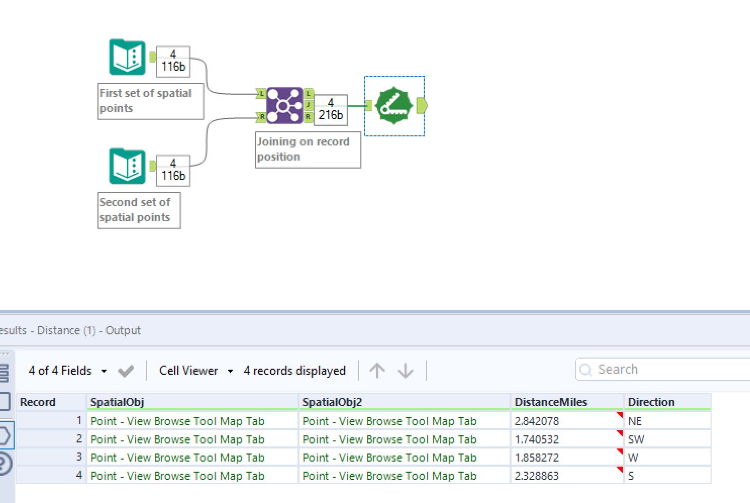
Pattern 2: The Sequential Method
This pattern is used when you want to find the distance between consecutive points within the same list, such as the distance between each stop on a delivery route. The Join method doesn't work here. Instead, we need to get the location of the next stop onto the row of the current stop. The Multi-Row Formula tool is perfect for this.
Let's see how this advanced technique works.
Distance between two points using Alteryx
This blog post from The Data School demonstrates a complete workflow for calculating distances between sequential bus stops. The key insight is its use of the Multi-Row Formula tool to prepare the data.
Focus on steps 3 and 4, titled 'Create a column with the Centroid for the next stop' and 'Create Distances'. Pay close attention to how the Multi-Row Formula tool is configured to create a new spatial object field. Note the importance of grouping to apply the logic correctly within each distinct route.
This Multi-Row Formula technique is a powerful addition to your Alteryx toolset, especially for pathing and route analysis. The key is using an expression like [Row+1:Centroid] and ensuring the new field's data type is set to SpatialObj.
3. Hands-On Practice
Let's apply the sequential method to a practical problem.
Scenario: You have a dataset tracking a single delivery truck's route, ordered by stop sequence. You need to calculate the travel distance between each consecutive stop.
- Open a new Alteryx workflow.
- Use a Text Input tool and enter the following data for the delivery route:
| StopID | Latitude | Longitude |
|---|---|---|
| 1 | 40.7128 | -74.0060 |
| 2 | 40.7195 | -73.9972 |
| 3 | 40.7295 | -73.9920 |
| 4 | 40.7350 | -74.0025 |
-
Add a Create Points tool. Configure it to create a point object for each stop, using
Longitudefor the X Field andLatitudefor the Y Field. Let's name the output fieldCentroid. -
Add a Multi-Row Formula tool. We will configure it to create a new field that contains the
Centroidof the next stop.- Click "Create New Field" and name it
NextStopCentroid. - Change the Type to SpatialObj.
- In the Expression box, enter
[Row+1:Centroid]. This tells Alteryx to take the value from theCentroidfield in the next row. - Leave "Group By" unchecked, as we only have one route.
- Click "Create New Field" and name it
-
Add a Distance tool after the
Multi-Row Formula.- Set the Point or Centroid Source to your
Centroidfield. - Set the Point, Line or Polygon Destination to your
NextStopCentroidfield. - Under Output Distance, you can leave the units as Miles or change them to Kilometers. For this exercise, we'll use the default straight-line distance.
- Set the Point or Centroid Source to your
-
Add a Browse tool to the output and run your workflow.
In the results, you should see a new "DistanceMiles" field. It will show the distance between Stop 1 and 2, Stop 2 and 3, and so on. Notice that the last row has a null distance, because there is no "next stop" after the final one. You could use a Filter tool to remove this row if needed.
4. Beyond Point-to-Point
Finally, it's worth noting that the Distance tool can also measure the distance from a point to the nearest edge of a line or polygon. This is useful for answering questions like, "How far is this customer from the boundary of their sales territory?" or "How far is this house from the nearest river?" You can explore this in the "Use Case 2: Point to Polygon" section of the Tool Mastery | Distance article we looked at earlier.
Conclusion
You have now mastered the Distance tool, a cornerstone of spatial analysis in Alteryx. You've learned how it functions and, more importantly, how to perform the necessary data preparation to make it work for both all-to-all and sequential comparisons.
Key Takeaways:
- The Distance tool calculates the distance between a source and destination spatial object located on the same record.
- It supports straight-line (ellipsoidal) distance, as well as driving distance and time (with the appropriate data pack).
- Data preparation is key. Use a Join/Append for comparing separate datasets and a Multi-Row Formula for calculating distances between sequential points in a single dataset.
This lesson concludes the Spatial Data Fundamentals module. You are now equipped with the foundational skills to create, visualize, manipulate, and measure spatial data.
Preview of the Next Lesson:
We're now ready to move into the Applied Spatial Analytics module. In our next lesson, we will expand on the concept of drive time by using the Trade Area tool to create drive-time polygons. This is a powerful technique for visualizing market reach and is frequently used in site selection and business catchment analysis.