Spatial Aggregation with the Spatial Process Tool

1. The Role of the Spatial Process Tool

The Spatial Process tool is a bit like a Swiss Army knife for spatial objects. It takes two spatial inputs (which can be individual objects or streams of objects) and performs a geometric operation to create a new spatial object output.

It has five distinct actions that determine how the two inputs interact. To get a clear definition of these actions, let's start with a brief reading.

As you just read, the five actions are:

• Combine Objects: Merges all input objects into a single, unified object.
• Cut 1st from 2nd: Creates an object that is the second object with the first object's area removed.
• Cut 2nd from 1st: Creates an object that is the first object with the second object's area removed.
• Create Intersection Object: Creates a new object representing only the area where both input objects overlap.
• Create Inverse Intersection Object: Creates a new object representing only the areas where the objects do not overlap.

For the purpose of aggregating data, the two most important actions to master are Combine Objects and Create Intersection Object.

2. Use Case 1: Combining Regions for Unified Analysis

Imagine you have several overlapping trade areas for stores in the same city. Before analyzing the total market, you might want to treat this entire area as one large region. The Combine Objects action is perfect for this. It takes all the input polygons and dissolves the internal boundaries, creating a single, clean polygon of the total area.

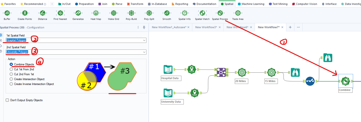
This action is used to aggregate the geographies themselves before you analyze the data within them.

3. Use Case 2: Aggregating Data via Intersection

This is the most powerful application of the Spatial Process tool for our learning goal. The Create Intersection Object action is the key to a technique called spatial apportionment (or areal interpolation).

Let's consider a common business scenario:

• You have a polygon representing a 10-minute drive-time trade area around your store.
• You have demographic data (like population or household income) aggregated at the ZIP Code level (as polygons).

A simple Spatial Match would tell you that your trade area intersects several ZIP Codes, but it wouldn't tell you how much it intersects them. Your trade area might cover 90% of one ZIP Code but only 5% of another. Simply summing the population of all intersected ZIP Codes would be highly inaccurate.

This is where Spatial Process comes in.

1. Find the Overlap: You use Spatial Process with the Create Intersection Object action. The inputs are your trade area polygon and the ZIP Code polygons. The output is a set of new, smaller polygons representing the exact areas where the trade area and ZIP codes overlap.
2. Calculate Proportion: Using the Spatial Info tool, you can calculate the area of these new intersection polygons. By comparing the intersection area to the original ZIP Code's total area, you can find the proportion of the ZIP Code that falls within your trade area.
3. Apportion the Data: You then multiply the total population of the ZIP Code by this proportion. If 40% of a ZIP Code's area is within the drive-time, you can estimate that 40% of its population is too.

This method allows for a much more accurate estimation of data within a custom-defined region.

The importance of the intersection action is a common theme in spatial analysis workflows.

4. Hands-On Practice: Estimating Overlapping Population

Let's build a workflow to apply the concept of spatial apportionment.

Scenario: Two retail stores, "Store A" and "Store B," have circular trade areas defined by a 2-mile radius. We know the total potential customer count within each full trade area. We need to estimate the number of potential customers in the overlapping "shared" market zone, assuming customer density is uniform.

1. Create Store Points:

   • Add a Text Input tool. Create two records, one for each store, with Latitude and Longitude.

     StoreName	Lat	Lon	Customers
     Store A	40.75	-73.99	10000
     Store B	40.76	-73.97	8000

   • Add a Create Points tool to convert these records into spatial point objects.

2. Create Trade Areas:

   • Add a Buffer tool after Create Points.
   • Configure it to create a buffer of 2 miles around each store's SpatialObj. This creates the two circular trade area polygons.

3. Isolate Each Trade Area:

   • We need to process each trade area separately to get its total area. Add a Filter tool after the Buffer.
   • Configure it to [StoreName] = "Store A".
   • Add another Filter tool from the same Buffer tool output. Configure it to [StoreName] = "Store B". You now have two separate streams.

4. Find the Intersection:

   • Add a Spatial Process tool.
   • Connect the 'True' output of the "Store A" filter to the left (1) input.
   • Connect the 'True' output of the "Store B" filter to the right (2) input.
   • In the configuration, select the Create Intersection Object action.

5. Calculate Areas:

   • Add a Spatial Info tool connected to the output of the Spatial Process tool. Check the box for Area (Square Miles). This will give you the area of the intersection.
   • Add another Spatial Info tool connected to the 'True' output of the "Store A" Filter tool (before it goes into Spatial Process). Also, check Area (Square Miles). This gives you the total area of Store A's trade area.

6. Join the Areas Together:

   • Add a Join tool. Connect the output of the "Intersection" Spatial Info tool to the left (L) input.
   • Connect the output of the "Store A" Spatial Info tool to the right (R) input.
   • Since there's no common field to join on, go to the configuration pane and uncheck all join fields. This will perform a Cartesian join, which is fine here since each input stream only has one record.

7. Estimate the Population:

   • Add a Formula tool after the Join.
   • Create a new column called Intersection_Customers.
   • The formula will be ([AreaSqMiles_L] / [AreaSqMiles_R]) * [Customers_R]. This calculates the ratio of the intersection area to Store A's total area, then multiplies it by Store A's total customer count.

8. Add Browse tools after the Formula tool and the Spatial Process tool to examine your final number and visualize the intersection polygon.

You have now successfully used spatial apportionment to estimate a value within an aggregated geographic region!

Conclusion

In this lesson, you moved beyond simply identifying objects within an area to actually aggregating and estimating data within complex geographic boundaries. You learned how the Spatial Process tool is essential for this task.

Key Takeaways:

• The Spatial Process tool manipulates spatial objects by performing geometric operations like combining them or finding their intersection.
• The Combine Objects action is used to merge multiple polygons into a single, unified region.
• The Create Intersection Object action is the foundation for spatial apportionment, a powerful technique to estimate data within a specific area of overlap.
• Spatial apportionment involves finding the intersection, calculating its proportional area relative to a larger known area, and applying that proportion to the data you want to estimate.

Preview of the Next Lesson:

So far in this module, we have created trade areas (Trade Area tool), found what's inside them (Spatial Match), and now learned how to aggregate data within them (Spatial Process). In the next lesson, we will put all these skills together to solve a complete business problem: conducting a site selection analysis to find the best location for a new store.