Understanding Hard Switching Power Losses

What is Hard Switching?

In an ideal world, a switch would turn on and off instantaneously. It would go from blocking all voltage (but with zero current) to conducting all current (but with zero voltage across it) in no time. In this ideal case, the power dissipated ($P=V\times I$) would always be zero.

Hard switching refers to the real-world scenario where we simply force the switch on and off without any special circuitry to manage the transition. Because the switch takes a finite time to change states, there is a period where both the voltage across it and the current through it are non-zero. This overlap is the source of switching loss.

Let's begin by reading a short article that introduces this concept and provides an excellent visual.

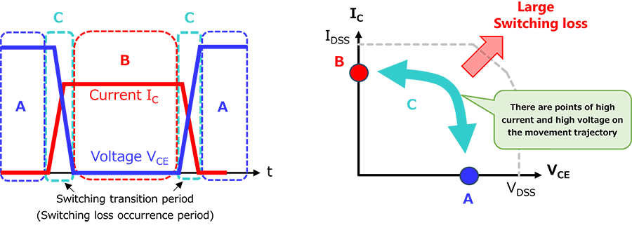
The key insight from that article is that power is dissipated during the transition. The following image breaks this down even further, showing the distinct phases of the turn-on and turn-off events.

The Switching Process in Detail

To understand why this overlap occurs, we need to look at the sequence of events during the turn-on and turn-off transitions. The internal capacitances of the MOSFET, which we discussed in the last lesson, play a starring role.

This next video provides a clear, step-by-step walkthrough of what happens inside a MOSFET as it switches an inductive load.

To summarize the video's key points:

• Turn-on: The gate voltage rises, turning the MOSFET on. The current begins to ramp up to the full load value. Only after the current has reached its peak does the drain-source voltage begin to fall to its low on-state value. During the time when current is rising and voltage is still high, power is lost.
• Turn-off: The process happens in reverse. The gate voltage falls, and the drain-source voltage begins to rise. Only after the voltage has reached the input voltage level does the drain current begin to fall. Again, there's a period where both voltage and current are high, causing power loss.

We can also visualize this on a current-voltage (I-V) plot. An ideal switch would just "teleport" between the ON state (high current, zero voltage) and the OFF state (zero current, high voltage). A hard-switched, real switch has to travel along a path between these two points, and this path traverses a region of high power dissipation.

From Instantaneous Spikes to Average Power Loss

The power spikes we've seen exist only for a few tens or hundreds of nanoseconds. However, they occur every single time the switch turns on or off. The total energy lost is the area under those power spikes. To find the average power loss, we multiply the energy lost per cycle by the number of cycles per second (the switching frequency).

Let's look at a simplified derivation. If we approximate the switching power waveforms as triangles, the area of each triangle (the energy) is roughly $\frac{1}{2}\times \text{base}\times \text{height}$.

• Height: The peak power, which is $V_{in}\times I_{load}$.
• Base: The switching time ($t_{on}$ or $t_{off}$).

So, the energy lost during one turn-on and one turn-off is:
$E_{SW}\approx \frac{1}{2}{V}_{in}{I}_{load}{t}_{on}+\frac{1}{2}{V}_{in}{I}_{load}{t}_{off}$

The average power loss, $P_{SW}$, is this energy multiplied by the switching frequency, $f_{sw}$:

$P_{SW}=E_{SW}\times f_{sw}\approx \frac{1}{2}{V}_{in}{I}_{load}(t_{on}+t_{off})f_{sw}$

This equation is fundamental. It tells us that switching loss is directly proportional to the switching frequency. This creates a core conflict in power supply design: designers want to increase frequency to use smaller inductors and capacitors (improving power density), but doing so directly increases switching losses and reduces efficiency. This is the trade-off that motivates the move to soft-switching topologies like ZVS.

A Deeper Dive: Gate Drive and Practical Trade-offs

The switching times, $t_{on}$ and $t_{off}$, are not fixed values. They are determined by how quickly the gate of the MOSFET can be charged and discharged. This speed is controlled by the gate driver circuit, most simply by a gate resistor.

You might think the solution is to use a very small gate resistor to switch as fast as possible. While this does reduce switching loss, it can create other problems. A very fast turn-on can worsen the effects of diode reverse recovery (an effect in the other switch in the half-bridge) and cause severe voltage ringing and electromagnetic interference (EMI).

This video demonstrates this exact trade-off by simulating a circuit with different gate resistors.

This highlights a key point for practical PCB reviews: the choice of gate drive components is a deliberate compromise between efficiency (low switching loss) and electrical integrity (low ringing and EMI).

Conclusion

In this lesson, you've learned about the central problem that modern power converters are designed to overcome.

Key Takeaways:

• Hard switching is the process of turning a switch on or off while there is simultaneously voltage across it and current through it.
• Because real switches have a finite transition time, this results in an overlap of the voltage and current waveforms.
• During this overlap, significant instantaneous power is dissipated in the switch ($P=V\times I$).
• The average switching power loss is proportional to the operating voltage, current, transition times, and most importantly, the switching frequency.
• This creates a fundamental trade-off between operating frequency (for smaller size) and efficiency.

You now understand the "what" and "why" of hard switching losses. In our next lesson, we will build on this by learning how to calculate these losses using parameters found directly in a MOSFET datasheet. This will give you the quantitative tools needed to evaluate the severity of this problem in a given design and to fully appreciate why ZVS is such an effective solution.