Graphing & Defining Polynomial, Exponential, & Logarithmic Functions

In our last lesson, we established the Cartesian coordinate system as the "canvas" for visualizing mathematical relationships. Now that we have this stage set, we can begin to draw the actors upon it. Today's lesson brings three of the most important families of functions to the forefront: polynomial, exponential, and logarithmic functions.

Your goal is to be able to define these functions and sketch their general behavior. This is not just an abstract exercise. These functions are the building blocks for modeling a vast array of real-world phenomena. Polynomials can approximate complex paths for a robot arm, exponential functions describe the growth of computational power (Moore's Law) and the decay of signals, and logarithms help us handle data that spans many orders of magnitude. A solid grasp of their shapes and properties is fundamental.

1. Polynomial Functions: The Shape of Complexity

We'll start with polynomials. You've encountered them before in forms like lines ( $y = m x + b$ , a polynomial of degree 1) and parabolas ( $y = a x^{2} + b x + c$ , a polynomial of degree 2). But what defines the entire family?

A polynomial is essentially a sum of terms, where each term consists of a coefficient multiplied by a variable raised to a non-negative integer power. To formalize this and understand the key vocabulary, let's turn to a video lecture.

Introduction to Polynomial Functions (Precalculus - College Algebra 27)

This video by Professor Leonard provides a clear and thorough introduction to what defines a polynomial function and its essential components.

Please watch the following two segments: This first part explains the general form of a polynomial and defines critical terminology: term, leading term, leading coefficient, degree, and constant term. Pay close attention to the importance of writing the polynomial in descending order of exponents. This second part covers the crucial rules for exponents in a polynomial (they must be non-negative integers) and explains why functions with radicals (fractional exponents) or variables in the denominator (negative exponents) are not polynomials. This also explains why the domain of any polynomial is always all real numbers.

To summarize the key takeaways from the video:

General Form: A polynomial function is written as $P (x) = a_{n} x^{n} + a_{n - 1} x^{n - 1} + \dots + a_{1} x + a_{0}$ .
Degree: The highest exponent, $n$ , which determines the function's overall complexity.
Leading Term: The term with the highest exponent, $a_{n} x^{n}$ . This single term is surprisingly powerful and dictates the graph's ultimate direction.
The Rule: Exponents must be whole numbers (0, 1, 2, ...). This ensures the graph is a single, smooth, unbroken curve.

Sketching Polynomials

Our goal isn't to plot a perfect graph by calculating dozens of points. Instead, we want to create a rough sketch that captures the function's essential features. The image below highlights the key characteristics we will use.

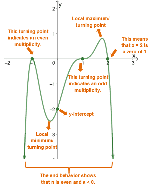
This graph illustrates the important features for sketching a polynomial: its end behavior, x-intercepts (zeros), the behavior at those zeros (related to multiplicity), local maximums and minimums (turning points), and the y-intercept.

To create such a sketch, we need a systematic approach. A fantastic resource from Paul's Online Math Notes outlines a process based on a few key ideas.

Algebra - Graphing Polynomials

This guide explains the theoretical tools needed to sketch a polynomial and lays out a clear step-by-step process.

Please read the following sections to understand the core concepts: Start with the introductory paragraphs and read down to the blue "Fact" box. Focus on the definitions of turning points and the relationship between the zeros of the polynomial and the x-intercepts of its graph. You'll find this material from the graph characteristics section. Now, read the "Fact" box itself and the explanation of the "Leading Coefficient Test". These two concepts are the engine of our sketching process. The fact about multiplicity tells you how the graph behaves at an x-intercept. An odd multiplicity means it crosses the x-axis, while an even multiplicity means it touches the axis and "bounces" off. The Leading Coefficient Test explains the end behavior—what the graph does as x goes to positive or negative infinity. This depends only on the degree (n) and the sign of the leading coefficient (a). Finally, read the four steps outlined in the blue box. This is our practical recipe for sketching.

The process can be summarized as:

Find the Zeros and their Multiplicity: Factor the polynomial to find where it equals zero. The multiplicity of each zero tells you if the graph crosses or bounces at that x-intercept.
Find the y-intercept: Simply calculate $P (0)$ .
Determine End Behavior: Use the Leading Coefficient Test.
Connect the Dots: Start from one end (using the end behavior), draw the curve through the intercepts (respecting the multiplicity behavior), and continue to the other end.

Now, let's see this process in action. The following video provides a concise visual demonstration.

Graphing Polynomial Functions Using End Behavior, Zeros, and Multiplicities

This video by Mario's Math Tutoring walks through the exact process you just read about, applying it to concrete examples.

Watch the following two examples to see how the theory is applied: The first example shows how to graph a polynomial that is already factored. This clearly demonstrates finding zeros, determining end behavior, and understanding multiplicities of 1. The second example starts with a polynomial that needs to be factored. It introduces a zero with a multiplicity of 2, so you can see the "bouncing" behavior at the x-intercept.

2. Exponential and Logarithmic Functions

Next, we move to two related families of functions that are crucial for modeling phenomena involving rapid change.

Exponential Functions: The Pace of Growth and Decay

An exponential function has the form $f (x) = a^{x}$ , where $a$ is a positive constant called the base. These functions appear everywhere, from modeling compound interest to population dynamics.

Exponential and logarithm functions

This document from Math Centre provides a concise overview of exponential and logarithmic functions and their graphs.

Please read the first part, Section 1. Exponential functions, found on pages 2-4. Pay close attention to: The general shape of the graph when the base is greater than 1 (a > 1), which represents exponential growth. The general shape when the base is between 0 and 1 (0 < a < 1), which represents exponential decay. The key properties summarized at the end of the section, such as the fact that the graph always passes through the point (0, 1).

A particularly important base is the number $e \approx 2.718$ . The function $f (x) = e^{x}$ is often called the exponential function due to its unique properties in calculus. Since $e > 1$ , its graph has the characteristic shape of exponential growth.

Logarithmic Functions: The Inverse of Exponentials

What if we know the result of an exponential process and want to find the input? For example, "How long will it take for my investment to double?" This is the question that logarithmic functions answer.

The function $f (x) = lo g_{a} (x)$ is the inverse of the exponential function $f (x) = a^{x}$ . The expression $lo g_{a} (x)$ asks: "What power do I need to raise the base $a$ to in order to get $x$ ?"

Let's return to the same PDF to explore their graphs.

Exponential and logarithm functions

We will continue with the Math Centre document.

Please read Section 2. Logarithm functions, found on pages 5-8. As before, focus on: The general shape of the graph when the base is greater than 1 (a > 1). The general shape when the base is between 0 and 1 (0 < a < 1). The key properties, such as the domain being restricted to positive numbers (x > 0) and the graph always passing through the point (1, 0).

Just as $e^{x}$ is the natural exponential function, $lo g_{e} (x)$ , usually written as $ln (x)$ , is the natural logarithm.

The Inverse Relationship

The connection between exponential and logarithmic functions as inverses is beautifully visualized by looking at their graphs together. A function and its inverse are always reflections of each other across the line $y = x$ .

This image shows that the graph of a logarithmic function (like y=log₂(x)) is a mirror image of its corresponding exponential function (y=2^x) across the diagonal line y=x. This visually confirms their inverse relationship.

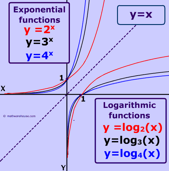
This reflection swaps the domain and range.

Exponential ( $a^{x}$ ): Domain is all real numbers, Range is $y > 0$ . Passes through (0, 1).
Logarithmic ( $lo g_{a} (x)$ ): Domain is $x > 0$ , Range is all real numbers. Passes through (1, 0).

Conclusion

In this lesson, you've learned to identify and sketch the three most common families of functions used in science and engineering.

Here are the key takeaways:

Polynomials are defined by their degree, and their graphs are smooth, continuous curves. Their shape is determined by end behavior (from the leading term) and the zeros with their multiplicities.
Exponential functions ( $a^{x}$ ) model rapid growth ( $a > 1$ ) or decay ( $0 < a < 1$ ). They all pass through (0, 1) and have a horizontal asymptote at the x-axis.
Logarithmic functions ( $lo g_{a} (x)$ ) are the inverses of exponentials. They model processes where quantities change over many orders of magnitude. They all pass through (1, 0) and have a vertical asymptote at the y-axis.

You now have a foundational visual library of function behaviors. In our next lesson, we will add another critical family to our toolkit: trigonometric functions. These functions are the language of everything that repeats or oscillates, from sound waves to the rotating joints of a robot, and they are indispensable in your journey toward engineering and AI.

Recommended resources