Hello! Welcome back to your course on low-frequency crypto trading.
In our first lesson, we established the conceptual foundation of momentum, defining it as the tendency for asset returns to exhibit positive autocorrelation over intermediate time horizons. This implies that past performance can be indicative of future performance.
Today, we will build directly on that foundation by focusing on the core component of that definition: the returns themselves. This lesson addresses the learning outcome: Calculate logarithmic and arithmetic returns for crypto assets and explain the implications of their statistical properties.
We will cover:
- The mathematical definitions and calculation of arithmetic (simple) and logarithmic (log) returns.
- The key properties of each, particularly their behavior over time and across assets.
- The statistical nature of crypto returns, moving beyond the common assumption of normality to understand concepts like "fat tails."
Mastering these concepts is a prerequisite for quantifying momentum and building any form of quantitative strategy.
1. Defining and Calculating Returns
The return of an asset is the most fundamental measure of its performance. There are two primary ways to calculate it: arithmetic and logarithmic.
1.1. Arithmetic (Simple) Returns
The arithmetic, or simple, return is the one most people are familiar with. It represents the percentage change in price over a single period.
The formula is:
where is the price at time and is the price at the previous time step.
While simple returns are intuitive for a single period, they are not additive over time. To find the total return over periods, you must compound them:
The following video provides a clear walkthrough of calculating simple and cumulative returns.
How To Calculate Stock Returns [Excel and in Python] - Returns, Cumulative Returns, Log returns
This video from Algovibes demonstrates how to calculate simple returns and, crucially, how to correctly calculate cumulative returns by compounding, contrasting it with the incorrect method of simple addition.
Watch from 00:30 to 04:14. Pay close attention to the distinction between summing returns (the wrong way) and compounding them (the right way) to find the total return over multiple periods.
1.2. Logarithmic (Continuously Compounded) Returns
Logarithmic returns are based on the concept of continuous compounding, which should be familiar from your physics and math background. Instead of compounding at discrete intervals (daily, monthly), we assume it happens infinitely often.
The formula for the log return is:
where is the natural logarithm.
To understand the origin of this formula and its link to continuous compounding, the next video provides an excellent derivation.
Log Returns in Finance: Continuous Compounding and Euler's Number (e) Explained
This video by Ryan O'Connell, CFA, FRM, derives the log return formula from first principles, starting with simple and discrete compounding and extending it to the continuous case using Euler's number, e.
Watch from the beginning to 10:03. This will walk you through the conceptual jump from discrete compounding (like a bank loan) to the continuous compounding assumed in liquid financial markets, leading directly to the log return formula.
The most important property of log returns is that they are time-additive. The total return over periods is simply the sum of the individual log returns:
To convert a total log return back to a simple return, you use the exponential function:
This time-additive property makes log returns incredibly convenient for statistical modeling and multi-period analysis.
2. Arithmetic vs. Log Returns: A Comparison
Choosing between simple and log returns involves a trade-off. The following article provides a concise summary of their pros and cons.
A brief overview on simple returns and log ...
This Medium article, 'A brief overview on simple returns and log ...', clearly lays out the advantages and disadvantages of both return types.
Read the sections 'Simple Returns' (Pros and Cons) and 'Log Returns' (Pros and Cons). Focus on the key distinction: simple returns are asset-additive, while log returns are time-additive.
Here is a summary of the key points:
| Feature | Arithmetic (Simple) Returns | Logarithmic Returns |
|---|---|---|
| Time Aggregation | Multiplicative: | Additive: |
| Portfolio Aggregation | Additive: | Not additive |
| Intuition | Highly intuitive (simple percentage change) | Less intuitive |
| Statistical Modeling | Difficult (product of random variables) | Easier (sum of random variables) |
| Symmetry | Asymmetric (e.g., +50% then -33% gets you back to start) | Symmetric (e.g., +ln(1.5) then -ln(1.5) gets you back to start) |
For small return values, arithmetic and log returns are nearly identical. The difference becomes significant with larger price changes, which are common in crypto markets.
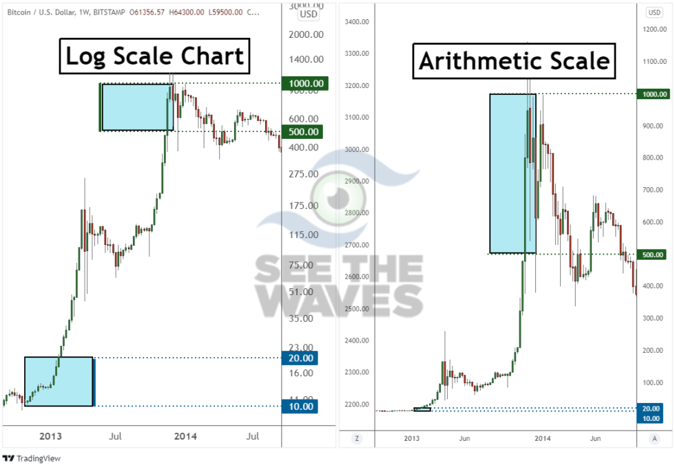
The choice of chart scaling—arithmetic vs. logarithmic—is a direct visual application of this concept. A logarithmic scale chart plots price changes such that equal vertical distances correspond to equal percentage changes, which is effectively visualizing log returns.
3. Statistical Properties and the "Fat Tail" Reality
In quantitative finance, it is often assumed that log returns are normally distributed. This assumption is mathematically convenient, as the sum of normally distributed variables is also normally distributed, which simplifies modeling.
However, for most financial assets, and especially for cryptocurrencies, this assumption is dangerously inaccurate. Real-world returns exhibit properties that a normal distribution fails to capture.
The Problem of "Fat Tails" (Leptokurtosis)
Financial returns are leptokurtic, meaning their distribution has "fat tails." This signifies that extreme events (both large gains and large losses) occur far more frequently than a normal distribution would predict. Assuming normality leads to a systematic underestimation of risk and the probability of "black swan" events.
The following reading explains this limitation and demonstrates it with Python code.
A brief overview on simple returns and log ...
This section of the Medium article 'A brief overview on simple returns and log ...' discusses the limitations of the normality assumption and shows how to test it.
Read the sections 'If we want to model returns using the normal distribution!' and 'Limitations'. Then, study the provided Python code blocks and the results of the Kolmogorov-Smirnov (KS) test. Note how both simple and log returns are shown to not fit a normal distribution, but they fit a Student's t-distribution much better.
As you saw in the article:
- Both simple and log returns for real stock data fail the KS test for normality. The low p-value allows us to reject the null hypothesis that the data comes from a normal distribution.
- A much better fit is achieved using the Student's t-distribution. This distribution has an additional parameter, degrees of freedom (), which controls the "fatness" of the tails. A lower means fatter tails. As , the t-distribution converges to the normal distribution.
- For financial modeling, especially in a volatile market like crypto, using a distribution that accounts for fat tails is crucial for realistic risk management and strategy evaluation.
4. Python Implementation
Calculating these returns in Python is straightforward using the pandas and numpy libraries.
- Simple Returns: The
pct_change()method in pandas is designed for this.import pandas as pd # Assuming 'df' is a DataFrame with a 'Close' column df['simple_return'] = df['Close'].pct_change() - Log Returns: You can use
numpy.log()in combination withshift().import numpy as np # Assuming 'df' is a DataFrame with a 'Close' column df['log_return'] = np.log(df['Close'] / df['Close'].shift(1))
The Python implementation section of the first video provides a good visual demonstration of these calculations.
How To Calculate Stock Returns [Excel and in Python] - Returns, Cumulative Returns, Log returns
This final clip from the Algovibes video shows how to implement the return calculations from the spreadsheet examples in Python using pandas and numpy.
Watch from 07:01 to 11:08. This will solidify your understanding of how to translate the formulas into practical code.
Conclusion
In this lesson, we have dissected the concept of returns, the fundamental input for any quantitative trading strategy.
Key Takeaways:
- Arithmetic (simple) returns are intuitive and asset-additive, making them useful for calculating portfolio performance at a single point in time.
- Logarithmic returns are time-additive, making them the standard for statistical modeling and multi-period analysis.
- For quantitative strategies like momentum, log returns are generally preferred due to their desirable mathematical and statistical properties.
- Crypto asset returns are not normally distributed. They exhibit fat tails, meaning extreme price moves are more common than a normal distribution suggests.
- The Student's t-distribution is a more realistic model for financial returns as it can account for fat tails. Acknowledging this is critical for robust risk management.
Now that we understand how to calculate returns from price data, the next logical step is to learn how to acquire that data efficiently and reliably.
In the next lesson, we will tackle the learning outcome: "Fetch historical OHLCV data for multiple crypto assets using REST APIs and handle exchange-specific rate limits and pagination." This will be a practical, hands-on lesson in building the data pipeline that will feed our future momentum calculations.