In our previous lesson, we mastered the chain rule, the mechanism for differentiating composite functions. We saw that it forms the backbone of backpropagation, the algorithm used to train neural networks. We also glimpsed how this concept extends to functions with multiple inputs, where the total influence of a variable is the sum of its effects through all possible paths.
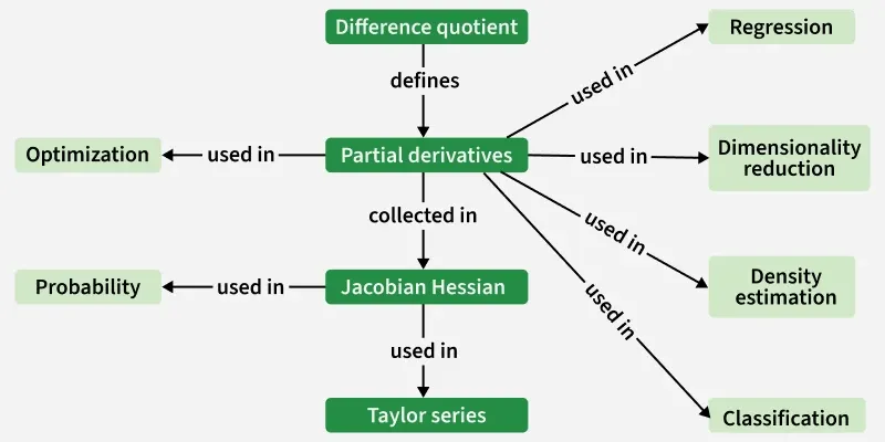
Today, we will formally step into the world of multivariable functions. This lesson focuses on partial derivatives, a tool for measuring how a function changes with respect to a single input variable, while all other inputs are held constant. This concept is central to your goal of building a PINN for radiotherapy. A radiation dose distribution, , is a function of three spatial variables. A partial derivative like tells you the rate of change of the dose as you move along the x-axis at a specific point, which is analogous to analyzing a single dose profile line. Understanding partial derivatives is the first step toward optimizing the complex functions that define neural networks.
From Surfaces to Slopes: The Core Idea
Functions with one variable, like , can be visualized as curves on a 2D plane. Their derivative, , gives the slope of the tangent line at any point. Functions with two variables, like , are visualized as surfaces in 3D space. How do we define "the slope" of a surface? The slope depends on the direction you're moving.
A partial derivative is the slope of the surface in a direction parallel to one of the coordinate axes.
The following video provides an excellent hands-on introduction. It starts by showing why we need partial derivatives for multivariable functions and then uses an interactive 3D plot to build a strong visual intuition.
What Partial Derivatives Are (Hands-on Introduction) — Topic 67 of Machine Learning Foundations
This video from Jon Krohn's "Machine Learning Foundations" series is perfect for building a visual and conceptual understanding of partial derivatives.
Please watch the following segments: Why we need partial derivatives: Start from the beginning and watch until this point. This sets the stage by connecting to multivariable functions in machine learning. Visualizing a surface: Continue from this timestamp. Here, the presenter uses a 3D plotter to explore the surface of the function z = x^2 - y^2. This "saddle" shape is a classic example. The partial derivative with respect to x: Now watch from this timestamp. This is the crucial part. Pay close attention to how "slicing" the 3D surface along the x-axis gives a 2D parabola, and how the partial derivative \frac{\partial z}{\partial x} is calculated by treating the other variable, y, as a constant. Also, note the new notation, \partial, which we call "del".
As the video showed, the key idea is to "freeze" all variables except the one you're interested in. By treating the other variables as constants, a multivariable calculus problem is temporarily simplified into a single-variable calculus problem that you already know how to solve.
The "Freeze and Differentiate" Method
Let's formalize the calculation process. The article below breaks it down into a clear, three-step method and provides worked examples.
Calculating Partial Derivatives
This article from APXML provides a concise guide to the mechanics of computing partial derivatives.
First, read the section explaining the process and walking through the first example, f(x,y)=x^2+y^3+4. This reinforces the concept you saw in the video. Next, read through the second example, g(w,b)=w^2b+5w−2b+7. This example is important because its structure, with variables multiplied together, is very similar to what you'll encounter in the equations for neural networks, where inputs are multiplied by weights.
The rules of differentiation (power rule, product rule, chain rule, etc.) all still apply. You just have to remember to apply them only to your target variable.
Let's see this applied to other types of functions you'll encounter, such as exponential functions, which are prevalent in physics models like radiation attenuation.
Partial Derivatives - Multivariable Calculus
This video by The Organic Chemistry Tutor provides a wealth of examples. We'll focus on just one for now.
Please watch the segment on exponential functions, from this timestamp. Notice how the chain rule is applied to the exponent. When finding the partial derivative with respect to x, the y^3 term inside the exponent is treated as a constant coefficient during the chain rule step.
From Theory to Code
You've now seen the theory and the manual calculation. Let's connect this back to Python. Since you are comfortable with NumPy, the following demonstration will feel familiar. It takes the same function from the first video, , and shows how to plot the function and its tangent lines, whose slopes are given by the partial derivatives.
What Partial Derivatives Are (Hands-on Introduction) — Topic 67 of Machine Learning Foundations
Let's return to Jon Krohn's video to see the Python implementation.
Code for ∂z/∂x: Watch the segment from this timestamp. Follow how the function f, the partial derivative del_z_del_x, and the plotting functions are defined. This is a practical demonstration of how the mathematical concept translates directly into code that visualizes the result. Theory for ∂z/∂y: Next, watch the conceptual explanation for the other partial derivative, from this timestamp. This will solidify your understanding by showing the same process applied to the other variable, y. The coding part for this is very similar, so we'll skip watching it, but feel free to explore it in the notebook if you're curious.
A Glimpse of the Gradient
We have learned to compute partial derivatives like and individually. In machine learning, these individual rates of change are almost always used together. They are collected into a vector called the gradient.
For a function , its gradient is written as (pronounced "nabla f" or "del f") and is defined as:
The gradient is a vector that points in the direction of the steepest ascent of the function at a given point. This is the single most important piece of information for optimization, as it tells us which way to adjust our model's parameters to increase (or decrease) a value, like the prediction error.
The following reading reinforces this final point.
Calculus — ML Glossary documentation
This cheatsheet provides a concise definition of the gradient and its relationship to partial derivatives.
Please read the introduction to Gradients and then follow the step-by-step example for the function f(x,z) = 2z^3x^2. Observe how the two partial derivatives are calculated separately and then assembled into the final gradient vector.
We will explore the properties and significance of the gradient in full detail in our next lesson.
Conclusion
In this lesson, we have moved from single-variable to multivariable calculus, a critical step toward understanding the mathematics of deep learning.
Key Takeaways:
- A partial derivative measures the rate of change of a multivariable function with respect to one variable, while all other variables are treated as constants.
- The notation for a partial derivative of with respect to is .
- Geometrically, a partial derivative represents the slope of a "slice" of the function's surface along a particular axis.
- To compute a partial derivative, you use the standard differentiation rules, but you "freeze" the variables you are not differentiating with respect to, treating them as constants.
- The individual partial derivatives of a function are collected into a vector called the gradient, denoted by .
In our next lesson, we will dive deep into the gradient vector. We will explore its properties, such as its direction and magnitude, and understand why it is the cornerstone of the optimization algorithms that train neural networks.