Chain Rule for Derivatives

Welcome back to our course. In our last lesson, we established the fundamental rules for finding derivatives of polynomial, exponential, and logarithmic functions. You might recall that when we differentiated functions like $e^{2 x}$ or $ln (x^{2} + 1)$ , we followed a two-step pattern: differentiate the "outer" function, then multiply by the derivative of the "inner" part.

Today, we will formalize this crucial pattern. This lesson is dedicated to the chain rule, which allows us to find the derivative of any composite function—a function built by nesting one function inside another. The chain rule isn't just another differentiation technique; it is the mathematical engine that powers the training of virtually all modern neural networks. A deep neural network is essentially a very complex composite function. The chain rule provides the mechanism, known as backpropagation, to calculate how a small adjustment to any parameter deep within the network affects its final prediction. Mastering this rule is a major step toward understanding how your dose prediction models will learn.

The Intuition: A Chain of Dependencies

Before diving into the formula, let's build an intuition for what the chain rule represents. Imagine a series of interconnected events where one rate of change influences another.

The StatQuest video below provides an excellent and memorable analogy involving weight, height, and shoe size to illustrate this concept.

The Chain Rule, Clearly Explained!!!

This video from StatQuest with Josh Starmer clearly explains the core idea of the chain rule using a simple, practical example.

Please watch the segment from the beginning up to this timestamp. Focus on how a change in the initial variable (weight) causes a change in the intermediate variable (height), which in turn causes a change in the final variable (shoe size). Notice that the overall rate of change is the product of the individual rates.

As the video demonstrates, if you have a chain of dependencies, the overall rate of change is found by multiplying the rates of change at each step in the chain. This is the essence of the chain rule.

The Formal Rule: "Outside-In"

Let's translate this idea into mathematical notation. A composite function has the form $h (x) = f (g (x))$ , where $g$ is the "inner" function and $f$ is the "outer" function.

A helpful way to visualize this is as a series of machines, where the output of the first machine, $g$ , becomes the input for the second machine, $f$ .

This diagram illustrates a composite function $f \circ g$. The input (a sphere) goes into machine $g$, its output (a red cube) goes into machine $f$, which produces the final output (a dodecahedron). The chain rule tells us how to find the overall rate of change by multiplying the rates of the individual machines.

The chain rule states that the derivative of the composite function $h (x)$ is:

h^{'} (x) = f^{'} (g (x)) \cdot g^{'} (x)

In Leibniz notation, if we let $u = g (x)$ and $y = f (u) = f (g (x))$ , the rule is expressed as:

\frac{d y}{d x} = \frac{d y}{d u} \cdot \frac{d u}{d x}

This beautifully mirrors the "multiplying rates" intuition. $\frac{d y}{d x}$ is the overall rate of change, which is the product of the rate of change of the outer function with respect to its input ( $\frac{d y}{d u}$ ) and the rate of change of the inner function with respect to its input ( $\frac{d u}{d x}$ ).

A common mental model for applying the rule is the "outside-in" or "onion peeling" method:

Differentiate the outermost function, leaving the inner function(s) unchanged inside it. This gives you the $f^{'} (g (x))$ part.
Multiply by the derivative of the inner function. This gives you the $g^{'} (x)$ part.

Applying the Chain Rule: Examples

Let's see this method in action. The following video walks through several examples, combining the chain rule with the power and trigonometric rules you already know.

Derivatives of Composite Functions: The Chain Rule

This video by Professor Dave Explains provides clear, step-by-step applications of the chain rule.

Please watch the following segments to see how the "outside-in" method works in practice: Introduction and Power Rule: Watch from the beginning to this timestamp. This section introduces the concept with \sqrt{x^2+1} and demonstrates the method. Trigonometric Functions: Watch from this timestamp. Pay close attention to the difference between differentiating \sin(x^2) and \sin^2(x). This highlights the importance of correctly identifying the outer and inner functions. Multiple Nested Functions: Finally, watch from this timestamp. This example with \sin(\cos(\tan(x))) shows how the chain rule is applied iteratively for functions with multiple layers, just like in a deep neural network.

As you saw, the rule can be applied repeatedly. For a function like $h (x) = f (g (k (x)))$ , the derivative is simply a longer chain of multiplications:

h^{'} (x) = f^{'} (g (k (x))) \cdot g^{'} (k (x)) \cdot k^{'} (x)

This is exactly what happens during backpropagation in a neural network with many layers.

A Glimpse of the Multivariable Chain Rule

So far, our functions have had a single input. However, in neural networks, a neuron's output typically depends on many inputs. The chain rule extends naturally to this multivariable setting.

Imagine a final value h depends on intermediate variables U1 and U2, which in turn both depend on an initial variable X1. The influence of X1 on h flows through two distinct paths.

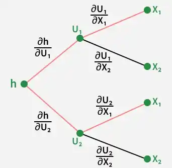
This tree diagram illustrates the multivariable chain rule. The total change in `h` with respect to `X1` is the sum of the changes propagated along the path through `U1` and the path through `U2`.

To find the total derivative of h with respect to X1, we must calculate the derivative along each path and then add them up. This "sum over all paths" principle is fundamental to how gradients are calculated in complex networks where one parameter can influence the final loss through many different connections.

The Chain Rule: Backbone of Backpropagation

This article provides a great analogy for the multivariable chain rule.

Please read the section on the multivariable rule. The "River Delta Analogy" provides a strong intuition for why we sum the contributions from different paths.

We will delve deeper into this when we cover partial derivatives and gradients in our next lesson.

From Math to Code: Automatic Differentiation

While it's crucial to understand the mechanics of the chain rule, you will rarely, if ever, compute these derivatives by hand for a real neural network. The complexity would be immense. Instead, we rely on a powerful technique called automatic differentiation (autodiff). Deep learning frameworks like PyTorch use autodiff to automatically and efficiently compute the derivatives of arbitrarily complex functions.

Autodiff is not a numerical approximation (like estimating the slope between two close points). It is the exact, algorithmic application of the chain rule. The software tracks every operation performed on your input data and uses this record to "backpropagate" the gradients by repeatedly applying the chain rule from the final output back to each input parameter.

To see this in action, we can use a library called MyGrad, which adds autodiff capabilities to NumPy. Since you're already familiar with NumPy, this should feel quite natural.

Automatic Differentiation

This resource introduces MyGrad and shows how it uses the chain rule to perform automatic differentiation.

First, read the section Introduction to MyGrad. This will show you the basic workflow of creating a Tensor, performing a calculation, and calling .backward() to compute the derivative. Next, read the section Seek and Derive. This part is key. It demonstrates how MyGrad can differentiate an extremely complex function and explicitly states: "It accomplishes this feat by dutifully applying the chain rule over and over, using a simple algorithm called “back-propagation”."

This bridge from manual calculus to automated computation is the key to practical deep learning. You provide the model architecture (the composite function), and the framework handles the calculus.

Conclusion

In this lesson, we have unpacked one of the most important concepts in the mathematics of deep learning.

Key Takeaways:

The chain rule is used to differentiate composite functions of the form $f (g (x))$ .
The rule is $(f (g (x)))^{'} = f^{'} (g (x)) \cdot g^{'} (x)$ , which can be thought of as "the derivative of the outer function (with the inner function intact) times the derivative of the inner function."
For functions with multiple layers of composition, the chain rule is applied iteratively, multiplying the derivatives at each step.
Backpropagation, the core algorithm for training neural networks, is a systematic application of the chain rule to compute how the model's error changes with respect to each of its parameters.
Automatic differentiation tools, built into frameworks like PyTorch, automate this process for us.

In our next lesson, we will build on this foundation and move into the world of multivariable functions. We will learn to compute partial derivatives and assemble them into a gradient vector, the object that will act as our guide for navigating the complex landscapes of neural network optimization.