Introduction
In our last lesson, we established a crucial decision framework: start with simple, rule-based systems and only move to machine learning when the problem's complexity demands it. We noted that a primary challenge in ML is building models that generalize well, avoiding the twin pitfalls of overfitting (memorizing the training data) and underfitting (failing to learn from it).
This lesson dives into the core theory that explains why this challenge exists. We will explore the bias-variance tradeoff, a fundamental concept that governs a model's ability to generalize. Understanding this tradeoff is essential for diagnosing model performance issues and is a cornerstone of ML theory frequently tested on certification exams.
By the end of this lesson, you will be able to explain what bias and variance are, how they create a tradeoff, and how this directly impacts whether your model underfits, overfits, or generalizes well to new, unseen data.
1. Defining Bias and Variance
At a high level, the total error of an ML model can be decomposed into three parts: bias, variance, and an irreducible error (random noise in the data that no model can eliminate). We will focus on the two components we can control: bias and variance.
A great way to visualize these concepts is with a target analogy. Imagine the center of the target is the "true" pattern in the data that we want our model to predict. Each shot at the target is a prediction made by a model trained on a different subset of our data.

Now let's solidify these definitions with a more concrete example.
Machine Learning Fundamentals: Bias and Variance
This video from StatQuest with Josh Starmer provides an excellent, intuitive explanation of bias and variance using a simple regression problem. It's one of the clearest introductions to the topic available.
Watch from the beginning to 05:16. Pay close attention to how the 'straight line' model and the 'squiggly line' model behave differently on the training and testing data. This is the key to understanding the two error types.
As the video demonstrates:
- Bias is the error introduced by a model's simplifying assumptions. A model with high bias makes strong assumptions about the data (e.g., the relationship is linear). It fails to capture the true underlying patterns, leading to underfitting. The "straight line" model had high bias because it couldn't capture the curve in the data, resulting in high error on both the training and test sets.
- Variance is the error from a model's sensitivity to small fluctuations in the training data. A model with high variance is too flexible and fits the noise in the training data, not just the signal. This leads to overfitting. The "squiggly line" model had low bias but high variance; it fit the training data perfectly but performed terribly on the test data because it had memorized the training points, including their noise.
2. The Tradeoff: Complexity vs. Error
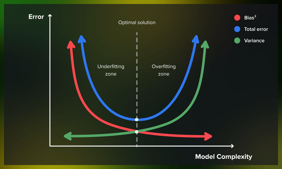
You might think the goal is to simply minimize both bias and variance. However, they are often in tension: decreasing one tends to increase the other. This is the bias-variance tradeoff.
The lever we use to navigate this tradeoff is model complexity.
- Simple Models (e.g., linear regression, shallow decision trees) have few parameters. They are rigid, making strong assumptions. This leads to high bias and low variance.
- Complex Models (e.g., deep neural networks, deep decision trees) have many parameters. They are highly flexible and can fit intricate patterns. This leads to low bias and high variance.
The relationship between complexity, bias, and variance is best shown with a classic graph.
This next short video segment provides a great verbal walkthrough of this exact curve.
Mastering Bias and Variance in Machine Learning Models | ML Optimization
Let's watch a clip from IBM Technology that explains this U-shaped curve and the concept of finding the 'sweet spot' for model complexity.
Watch from 02:26 to 04:26. Focus on how the total error is a combination of bias and variance, and why the lowest total error is not at the point of lowest bias or lowest variance.
The key takeaway is that your goal is not to achieve zero training error. That would likely mean you have a high-variance model that is severely overfit. Your goal is to find the model complexity that results in the lowest possible error on unseen data (i.e., the test set).
3. Diagnosing Bias vs. Variance Issues
You now understand the theory. But in practice, how do you know if your model is suffering from high bias or high variance? You compare its performance on the training set versus the validation/test set.
| Scenario | Training Error | Validation/Test Error | Diagnosis | Primary Problem |
|---|---|---|---|---|
| 1 | High | High | High Bias | Underfitting |
| 2 | Low | High | High Variance | Overfitting |
| 3 | Low | Low | Good Balance | Good Generalization |
| 4 | High | Very High | High Bias & High Variance | Severe problem, often data-related |
This table is a critical diagnostic tool. For the exam, you must be able to look at training and validation metrics and immediately identify the likely problem.
To get a more formal definition and a consolidated view, please review the following text.
Bias-Variance Tradeoff in Machine Learning - Great Learning
This article from Great Learning provides clear, concise definitions and a helpful summary table. It also introduces the mathematical representation of total error.
Read from the 'Introduction' through to the end of 'The Bias-Variance Tradeoff in Machine Learning'. Pay special attention to the table in the 'Bias vs Variance: A Comparative Analysis' section, as it's an excellent summary for exam revision.
4. Strategies for Managing the Tradeoff
Once you've diagnosed the problem, you can apply specific strategies to fix it. This is a crucial skill for an ML engineer.
If you have high bias (underfitting):
Your model is too simple. You need to increase its complexity.
- Use a more complex model: Switch from linear regression to a Gradient Boosted Tree or a neural network.
- Add more features: Engineer new features that might help the model find more patterns.
- Decrease regularization: Regularization techniques intentionally add bias to reduce variance. Reducing them can help with an underfitting problem. (We will cover regularization in detail later).
If you have high variance (overfitting):
Your model is too complex for the amount of data you have. You need to reduce its effective complexity or give it more data to learn from.
- Get more training data: This is often the most effective solution. More data helps the model learn the true signal and ignore the noise.
- Reduce model complexity: Use a simpler model, reduce the depth of decision trees, or use fewer layers/neurons in a neural network.
- Apply regularization: This penalizes model complexity, forcing it to be simpler and reducing its variance.
- Use feature selection: Remove irrelevant or noisy features.
This next resource provides excellent practical examples and clarifies common misconceptions.
Bias-Variance Tradeoff: How Models Fail in Production - DataCamp
The article 'Bias-Variance Tradeoff: How Models Fail in Production' from DataCamp gives a great walkthrough of these concepts with a practical rental price prediction example. It also clarifies the link between different algorithm types and their inherent bias/variance tendencies.
Please read the following sections: 'A Simple Bias-Variance Tradeoff Example': This makes the concept concrete. 'Bias-Variance Tradeoff in Machine Learning Models': This connects specific algorithms (like linear models vs. neural nets) to the tradeoff. 'Bias-Variance Tradeoff vs. Overfitting and Underfitting': This explicitly clarifies the relationship between the terms. 'Practical Tips for Interpreting Model Performance': This summarizes the diagnostic process.
Conclusion
You have now explored the bias-variance tradeoff, one of the most important guiding principles in machine learning. It provides the theoretical foundation for understanding why models overfit or underfit and gives you a framework for diagnosing and addressing these common failures.
Key Takeaways:
- A model's total error on unseen data is a combination of bias, variance, and irreducible error.
- Bias is error from wrong assumptions, leading to underfitting. Simple models have high bias.
- Variance is error from sensitivity to the training data, leading to overfitting. Complex models have high variance.
- The tradeoff means that decreasing one type of error often increases the other, controlled by model complexity.
- You can diagnose the problem by comparing training error vs. test error. High/High suggests high bias; Low/High suggests high variance.
- You manage the tradeoff by adjusting model complexity, adding data, or using techniques like regularization.
In this lesson, we talked about "error" as a general concept. But to train a model, we need to quantify this error precisely. The next lesson, "Describe common loss functions (e.g., MSE, cross-entropy) and when each applies," will do just that. We will examine the specific mathematical functions used to measure a model's error during training, which is the very quantity that optimization algorithms like gradient descent work to minimize.