Ray-Sphere Intersection: The Quadratic Formula Approach

Setting the Stage: The Mathematics of Rays and Spheres

Before we find out where a ray and sphere intersect, we need to define them mathematically.

1. The Ray

As we've discussed, a ray can be described by a parametric equation. It has an origin point O and a direction vector d. Any point P along the ray can be found using a scalar parameter t:

$\mathbf{P}(t)=\mathbf{O}+t\mathbf{d}$

Here, t represents the distance along the ray from its origin. For our purposes, we are interested in intersections that happen in front of the camera, so we only care about positive values of t.

2. The Sphere

The equation for a sphere is also straightforward. A sphere is defined by its center point C and its radius r. Any point P on the surface of the sphere satisfies the condition that its distance from the center C is equal to r.

In vector notation, this is expressed as:

$||\mathbf{P}-\mathbf{C}||=r$

To avoid dealing with square roots, we usually work with the squared form of this equation. Since the squared length of a vector is equal to the dot product of the vector with itself (||\mathbf{v}||^2 = \mathbf{v} \cdot \mathbf{v}), the equation for a sphere becomes:

$(\mathbf{P}-\mathbf{C})\cdot (\mathbf{P}-\mathbf{C})=r^2$

This equation states that any point P that satisfies this condition lies on the sphere's surface.

The Intersection: Combining the Equations

The core of our task is to find out if there's any point that lies on both the ray and the sphere. In other words, we're looking for a value of t where the point on the ray, P(t), satisfies the sphere's equation.

To find this t, we simply substitute the ray's equation into the sphere's equation. This is the central algebraic step of the process.

To see this derivation explained with clear, step-by-step visuals, we'll watch a detailed video. It uses a 2D ray-circle intersection for simplicity, but the algebraic steps are identical for the 3D case we'll be implementing.

Unpacking the Derivation in 3D

The video provided a great intuition in 2D. Now, let's formalize the result for our 3D case using the vector notation from our main guide, Ray Tracing in One Weekend. This is the form we'll use in our code.

Let's restate the substitution:

1. Start with the sphere equation:
   $(\mathbf{P}-\mathbf{C})\cdot (\mathbf{P}-\mathbf{C})=r^2$
2. Substitute the ray equation, $\mathbf{P}(t)=\mathbf{O}+t\mathbf{d}$, into P:
   $((\mathbf{O}+t\mathbf{d})-\mathbf{C})\cdot ((\mathbf{O}+t\mathbf{d})-\mathbf{C})=r^2$
3. Rearrange the terms to group the unknown t. Let the vector from the sphere's center to the ray's origin be $(\mathbf{O}-\mathbf{C})$:
   $(t\mathbf{d}+(\mathbf{O}-\mathbf{C}))\cdot (t\mathbf{d}+(\mathbf{O}-\mathbf{C}))=r^2$
4. Expand the dot product using the distributive property ((A+B)·(A+B) = A·A + 2A·B + B·B):
   $(t\mathbf{d}\cdot t\mathbf{d})+2(t\mathbf{d}\cdot (\mathbf{O}-\mathbf{C}))+((\mathbf{O}-\mathbf{C})\cdot (\mathbf{O}-\mathbf{C}))=r^2$
5. Gather the coefficients of t to reveal the quadratic form at² + bt + c = 0:
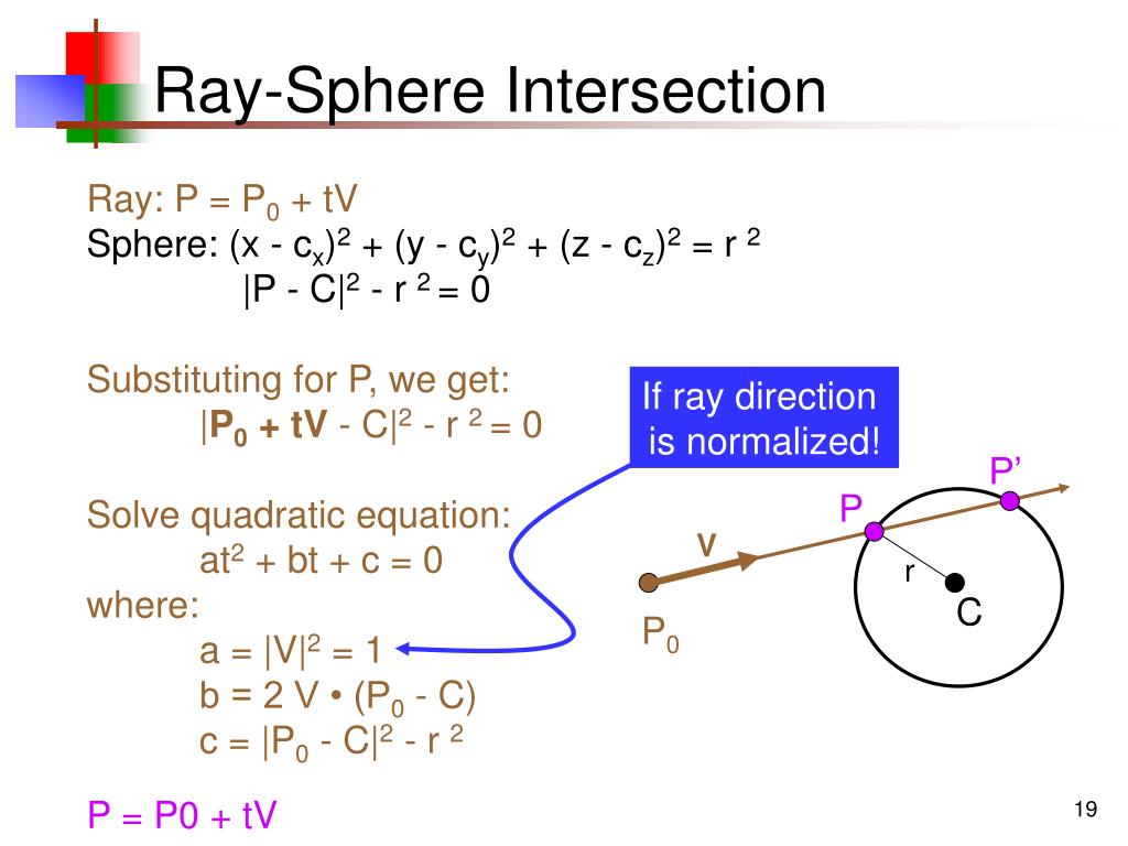
   $t^2(\mathbf{d}\cdot \mathbf{d})+t(2\mathbf{d}\cdot (\mathbf{O}-\mathbf{C}))+((\mathbf{O}-\mathbf{C})\cdot (\mathbf{O}-\mathbf{C}))-r^2=0$

This is it! This is our quadratic equation for t. The coefficients a, b, and c are all scalar values that we can compute from the known properties of our ray and sphere:

• $a=\mathbf{d}\cdot \mathbf{d}$
• $b=2\mathbf{d}\cdot (\mathbf{O}-\mathbf{C})$
• $c=(\mathbf{O}-\mathbf{C})\cdot (\mathbf{O}-\mathbf{C})-r^2$

The following image provides a great visual summary of this entire derivation.

Solving for t: The Quadratic Formula

Now that we have a standard quadratic equation, we can solve for t using the familiar quadratic formula:

$t=\frac{-b\pm \sqrt{b^2-4ac}}{2a}$

The most important part of this formula for ray tracing is the term inside the square root, called the discriminant ($\Delta$):

$\Delta =b^2-4ac$

The value of the discriminant tells us exactly how many times the ray intersects the sphere, directly connecting the algebra to the geometry:

• If $\Delta <0$: There are no real solutions for t. The ray misses the sphere completely.
• If $\Delta =0$: There is exactly one real solution for t. The ray grazes the sphere at a single point, i.e., it is tangent.
• If $\Delta >0$: There are two distinct real solutions for t. The ray passes through the sphere, intersecting it at an entry and an exit point.

For rendering, we are typically interested in the smallest positive t value, as this represents the first intersection point the ray encounters.

An Algebraic Simplification

The authors of Ray Tracing in One Weekend make a small algebraic simplification that cleans up the code nicely. Notice that the b coefficient has a factor of 2. If we let b = 2h, the quadratic formula simplifies:

$t=\frac{-2h\pm \sqrt{(2h{)}^2-4ac}}{2a}=\frac{-2h\pm 2\sqrt{h^2-ac}}{2a}=\frac{-h\pm \sqrt{h^2-ac}}{a}$

From our original b, we can find h:
$b=2\mathbf{d}\cdot (\mathbf{O}-\mathbf{C})$, so $h=\mathbf{d}\cdot (\mathbf{O}-\mathbf{C})$.

The new, simpler discriminant is just $h^2-ac$. This form is slightly more efficient as it reduces the number of multiplications. We will use this refined version when we implement our hit_sphere function.

To see the full derivation and C++ implementation details using this simplified formula, you can refer to the following resource. We won't be writing the code today, but seeing how the math is structured will be very helpful for the next lesson.

Conclusion

Excellent work! You've now walked through the complete derivation of one of the most fundamental algorithms in ray tracing. This is a perfect example of how the abstract principles of analytical geometry and linear algebra are applied to create tangible visual results.

Key Takeaways:

• Ray-sphere intersection is found by substituting the ray's parametric equation into the sphere's implicit equation.
• This substitution results in a quadratic equation of the form $a{t}^2+bt+c=0$, where t is the distance along the ray.
• The coefficients a, b, and c are scalars computed from dot products of the ray's and sphere's vectors.
• The discriminant ($b^2-4ac$) of the quadratic formula determines the number of intersection points (0, 1, or 2), corresponding to a miss, a tangent hit, or a pass-through.

Next Steps

We have done the hard part—the math! In the next lesson, we will translate this derivation into code. We will implement a function that takes a ray and a sphere and returns true or false depending on whether they intersect. This will allow us to render our very first 3D object.